USearch Molecules: Searchable Dataset of 28 Billion Chemical Embeddings on AWS ⚗️

TLDR: I’ve finally finished a project that involved gathering 7 billion small molecules, each represented in SMILES notation and having fewer than 50 “heavy” non-hydrogen atoms. Those molecules were “fingerprinted”, producing 28 billion structural embeddings, using MACCS, PubChem, ECFP4, and FCFP4 techniques. These embeddings were indexed using Unum’s open-source tool USearch, to accelerate molecule search. This extensive dataset is now made available globally for free, thanks to a partnership with AWS Open Data. You can find the complete data sheet and scripts for data visualization on GitHub.

Introducing the “USearch Molecules” dataset!

This dataset is notable for its sheer size and might be one of the largest datasets of embeddings available. It encompasses approximately 2.3 TB of data across 7,000 files, housed in the s3://usearch-molecules bucket in AWS’s us-west-2 region.

1

aws s3 ls --no-sign-request s3://usearch-molecules # to list bucket contents

What sets this dataset apart is not just its size, making it a potential candidate for upcoming editions of the Big ANN Benchmark, but also its unique composition compared to typical AI-generated embeddings. In Cheminformatics, a different approach is used: subgraph-matching techniques to derive structural properties of molecule graphs, leading to binary arrays representing these features. Over the past five months of working with this and related datasets, I’ve discovered several interesting insights applicable in other areas. The development process was iterative, optimizing speed and accuracy and finding a balance between the two.

• Speeding Up Indexing and Retrieval:
  • Invoking AVX-512 VPOPCNTQD Assembly instruction for computing Jaccard distance, achieving a 56x speed improvement over SciPy for vectors of any length.
  • Employing the Numba JIT compiler with bit-hacks to tune the distance metric for a specific number of dimensions in Python, further accelerating search by around 30%.
• Enhancing Search Accuracy with Hybrid Embeddings:
  • Combining different embeddings to lower error rates by up to 3.5x.
  • Developing similarity metrics with conditional thresholds to accelerate indexing and search by more than 60%, maintaining over 100,000 vectors/second throughput.
  • Adjusting HNSW hyper-parameters to balance throughput and accuracy, achieving 99% “recall at one”, handling 3,000 requests per second over 1 billion entries.

Ready to explore more? Let’s dive in!

Background and Motivation

The inspiration for this project came from my colleagues, the creators of the BARTSmiles paper. In their research, they developed a generative Transformer model. This model can predict molecular properties using only a SMILES string. For example, consider Melatonin, a well-known molecule. Its chemical formula is C₁₃H₁₆N₂O₂, but in SMILES notation, it is represented as:

CC(=O)NCCC1=CNc2c1cc(OC)cc2

Given such a SMILES string, the model can predict a range of molecular properties. These include Lipophilicity, which is a molecule’s tendency to combine with fats over water, and Genotoxicity, which refers to the potential of chemicals to harm cellular genetic material.

Additionally, the model excelled in tasks like retrosynthesis and chemical reaction prediction. This is particularly relevant to AI researchers as it parallels sequence-to-sequence modeling tasks. However, their dataset was vast and complex, posing a challenge in navigation. This is where our interests intersected and I started tuning my libraries for molecule retrieval.

Gathering Data

For this project, I have compiled three datasets:

• 115'034'339 molecules from the “PubChem” dataset.
• 977'468'301 molecules from the “GDB-13” dataset.
• 6'039'411'651 molecules from the Enamine “Real” dataset.

In total, this amounts to over 7 billion molecules. Handling data at this scale can be challenging, as anomalies are common, and pipelines can become complicated. For instance, a simple task like reading a .smi file with newline-delimited molecule descriptions could take hours using basic Python methods:

1

open("molecules.smi", "r").readlines()

To tackle this, I’ve extended my strings processing library, known as Stringzilla 🦖, covered in a previous post. Having a fast Str class and a memory-efficient Strs array addressing large memory-mapped files saved me over $10,000 in processing costs.

Using StringZilla, I normalized and shuffled the data, then split it into Parquet files. Each file contains up to 1 million molecules. For parsing SMILES strings into molecular graphs and computing fingerprints, I employed two libraries: RDKit in Python and Chemistry Development Kit (CDK) in Java. The result was a series of Parquet files containing the original SMILES string and multiple binary columns.

Understanding Molecule Fingerprints

Interpreting SMILES strings is not straightforward for humans or computers. A more intuitive approach is to depict molecules as a network of atoms and bonds akin to a graph. For instance, Melatonin’s structure includes an indole ring. This is a combination of a benzene ring (a hexagon shape) and a pyrrole ring (a pentagon shape).

Comparing such representation, however, is computationally expensive. In mathematical terms, this involves solving graph isomorphism and subgraph isomorphism problems. These are complex challenges known as NP-intermediate and NP-complete, respectively. Fortunately, chemists have developed heuristics to circumvent expensive isomorphism checks. In cheminformatics, a common practice is to create “fingerprints” of molecules. These fingerprints are arrays filled with zeros and ones. Each ‘1’ in this array indicates the presence of a particular molecular feature, often a specific sub-structure.

Consider this “MACCS Key” as an example:

00000000000000000000000000000000000000000000000000000000000000000100000000000000001100000011110010001100110010110100111001000111000100000100001100010101111111111111110

It represents 44 set bits, each corresponding to a pattern in the “SMiles ARbitrary Target Specification” (SMARTS), including key features like:

• Benzene Ring: A six-membered aromatic ring. The SMARTS pattern #163 (*1~*~*~*~*~*~1) identifies the six-membered structure, while #162 (a) indicates its aromatic nature.
• Pyrrole Ring: A five-membered aromatic ring containing nitrogen, identified by #96 (*1~*~*~*~*~1) for its five-membered structure and #121 ([#7;R]) for the presence of

You can use the following snippet to log the features of a specific molecule:

1
2
3
4
5
6
7
8

from rdkit import Chem
from rdkit.Chem import MACCSkeys

molecule = Chem.MolFromSmiles('CC(=O)NCCC1=CNc2c1cc(OC)cc2')
fingerprint = MACCSkeys.GenMACCSKeys(molecule) # produces MACCS fingerprint
for i, x in MACCSkeys.smartsPatts.items(): # iterates through patterns
    if fingerprint[i]: # check if that key is enabled
        print(f"{i}: {x}") # prints 44 lines

Exploring Different Molecule Fingerprints

In the realm of cheminformatics, various methods exist for generating molecule fingerprints. For this project, I focused on four types:

• MACCS Keys: These are Molecular ACCess System keys, featuring 166 dimensions. They provide a standard way to represent molecular structures for comparison.
• PubChem Fingerprints: These involve substructure fingerprints with 881 dimensions, commonly used for detailed representation in the PubChem database.
• ECFP4: Standing for Extended Connectivity Fingerprint of diameter 4, this method offers 2048 dimensions. It’s well-suited for capturing intricate molecular details.
• FCFP4: Known as Functional Class Fingerprint of diameter 4, also with 2048 dimensions, it focuses more on the functional groups within molecules.

It’s also common to see ECFP and FCFP with a diameter of 6, and their sizes can vary between 1024, 2048, and 4096 bits. The FCFP’s generation process is akin to that of ECFP, but it starts by categorizing atoms into functional classes, thereby emphasizing the significance of functional groups in molecular structures. This feature is particularly beneficial in predictive modeling and similarity assessments in pharmacological research.

Developing a Proof of Concept

Despite their diverse origins, these fingerprints share a common ground when it comes to comparison – they are all typically evaluated using the Tanimoto coefficient, a variation of the Jaccard distance applied to bit-strings:

$$ Jaccard(A, B) = 1 - \frac{|A \cap B|}{|A \cup B|} $$

Creating a prototype using the Jaccard distance in NumPy is straightforward.

1
2
3
4
5
6
7
8

import numpy as np

def jaccard(a: np.ndarray, b: np.ndarray) -> float:
    a = np.unpackbits(a.view(np.uint8))
    b = np.unpackbits(b.view(np.uint8))
    ands = np.logical_and(a, b).sum()
    ors = np.logical_or(a, b).sum()
    return 1 - ands / ors

By integrating this with rdkit, we transition from molecular structures to bit-strings, applying our similarity function to molecules like melatonin, methoxyethane, and ethanol.

 1
 2
 3
 4
 5
 6
 7
 8
 9
10
11

import numpy as np
from rdkit import Chem
from rdkit.Chem import MACCSkeys

smiles = ['CC(=O)NCCC1=CNc2c1cc(OC)cc2', 'CCOC', 'CCO']
molecules = [Chem.MolFromSmiles(x) for x in smiles]
fingerprints = [np.packbits(MACCSkeys.GenMACCSKeys(x)) for x in molecules]

melatonin_methoxyethane_distance = jaccard(fingerprints[0], fingerprints[1]) # 0.98
melatonin_ethanol_distance = jaccard(fingerprints[0], fingerprints[2]) # 0.99
methoxyethane_ethanol_distance = jaccard(fingerprints[1], fingerprints[2]) # 0.39

With these components in place, integrating them with the USearch vector search engine allowed us to prototype a functional search system:

1
2
3
4
5
6
7

from usearch.index import Index, MetricKind

index = Index(ndim=166, metric=MetricKind.Tanimoto)

keys = [hash('melatonin'), hash('methoxyethane'), hash('ethanol')]
index.add(keys, fingerprints)
matches = index.search(fingerprints[-1], 1)

This system successfully identified ethanol as the closest match in our index to ethanol, confirming the functionality of our prototype. Yet, our knowledge of the dataset opens doors to further optimizations, each tailored to leverage specific characteristics of the data.

Speed Optimizations

Hardware-Specific Tuning with AVX-512

A regular reader of my “Less Slow” blog is probably thinking - “When you’re a hammer, everything looks like a nail.”

A baseline C++ implementation of the Jaccard distance may look like this:

 1
 2
 3
 4
 5
 6
 7
 8
 9
10

#include <bitset>

float jaccard(std::uint8_t const* a, std::uint8_t const* b, std::size_t words) noexcept {
    float and_count = 0;
    float or_count = 0;
    for (std::size_t i = 0; i != words; ++i)
        and_count += std::bitset<8>(a[i] & b[i]).count(),
        or_count += std::bitset<8>(a[i] | b[i]).count();
    return 1 - and_count / or_count;
}

This will not result in the best Assembly, even using the newest compiler. Using Intel’s 4th Gen Xeon Scalable CPUs, codenamed Sapphire Rapids, we know the instructions optimal assembly will contain:

• The vpopcntq instruction computes population counts of bit-sets in just 3 cycles.
• Two vmovdqu8 zmm loads can run simultaneously, taking 10 cycles.
• Masked loads like vmovdqu8 zmm {z} can bypass the tail loop.
• The bzhi instruction computes the {z} mask in only 1 CPU cycle.
• Instructions such as vpandd, vpord, and vpaddq each take merely 1 cycle.

Here’s an example of how this looks in a production C 99 codebase using GCC intrinsics:

 1
 2
 3
 4
 5
 6
 7
 8
 9
10
11
12
13
14
15
16
17
18
19
20
21
22
23
24
25
26
27

__attribute__((target("avx512vpopcntdq,avx512vl,avx512bw,avx512f,bmi2")))
inline static simsimd_f32_t simsimd_avx512_b8_jaccard(simsimd_b8_t const* a, simsimd_b8_t const* b, simsimd_size_t n_words) {
    __m512i intersection_vec = _mm512_setzero_si512(), union_vec = _mm512_setzero_si512();
    __m512i a_vec, b_vec;

simsimd_avx512_b8_jaccard_cycle:
    if (n_words < 64) {
        __mmask64 mask = _bzhi_u64(0xFFFFFFFFFFFFFFFF, n_words);
        a_vec = _mm512_maskz_loadu_epi8(mask, a);
        b_vec = _mm512_maskz_loadu_epi8(mask, b);
        n_words = 0;
    } else {
        a_vec = _mm512_loadu_epi8(a);
        b_vec = _mm512_loadu_epi8(b);
        a += 64, b += 64, n_words -= 64;
    }
    __m512i and_vec = _mm512_and_si512(a_vec, b_vec);
    __m512i or_vec = _mm512_or_si512(a_vec, b_vec);
    intersection_vec = _mm512_add_epi64(intersection_vec, _mm512_popcnt_epi64(and_vec));
    union_vec = _mm512_add_epi64(union_vec, _mm512_popcnt_epi64(or_vec));
    if (n_words)
        goto simsimd_avx512_b8_jaccard_cycle;

    simsimd_size_t intersection = _mm512_reduce_add_epi64(intersection_vec),
                   union_ = _mm512_reduce_add_epi64(union_vec);
    return (union_ != 0) ? 1 - (simsimd_f32_t)intersection / (simsimd_f32_t)union_ : 0;
}

This implementation was 56 times faster than the SciPy implementation in specialized micro-benchmarks:

• SciPy distances… up to 200x faster with AVX-512 & SVE.
• Python, C, Assembly - 2'500x Faster Cosine Similarity.
• GCC Compiler vs Human - 119x Faster Assembly.

Problem-Specific Tuning with Numba

Our previous implementation works well for general cases, but we can do better with more specific information. For example, with MACCS, we know our vectors are precisely 166 bits long. This can be broken down as:

• 20x 8-bit words, with an additional 6 bits extending into a 21st word.
• 5x 32-bit words, with an additional 6 bits extending into a 6th word.

Knowing these specifics, we can avoid the for loop by unrolling the iterations over 8-bit words 21 times. Alternatively, we can pad each vector to a more computationally efficient 24-byte length, using 32-bit words for faster processing. With Numba, our distance metric takes this form:

 1
 2
 3
 4
 5
 6
 7
 8
 9
10
11
12
13
14

from numba import cfunc, types, carray, njit

numba_signature = types.float32(types.CPointer(types.uint32), types.CPointer(types.uint32))

@cfunc(numba_signature)
def tanimoto_maccs(a, b):
    a_array = carray(a, 6)
    b_array = carray(b, 6)
    ands = 0
    ors = 0
    for i in range(6):
        ands += word_popcount(a_array[i] & b_array[i])
        ors += word_popcount(a_array[i] | b_array[i])
    return 1 - types.float32(ands) / ors

This code needs the word_popcount function, which counts the number of set bits in a 32-bit word. A simple Python implementation might look like this:

1
2

def word_popcount(word: int) -> int:
    return bin(word).count('1')

On the bright side, modern CPUs can perform this operation in a single CPU cycle, and we don’t need to allocate any strings. On the other side, Numba doesn’t expose this part of LLVM functionality. So we need to use a bit-hack to implement a population count:

1
2
3
4
5
6

@njit("int_(uint32)")
def word_popcount(word):
    word = word - ((word >> 1) & 0x55555555)
    word = (word & 0x33333333) + ((word >> 2) & 0x33333333)
    c = types.uint32((word + (word >> 4) & 0xF0F0F0F) * 0x1010101) >> 24
    return c

Combining all these elements, we pass them to USearch as a CompiledMetric:

 1
 2
 3
 4
 5
 6
 7
 8
 9
10

from usearch.index import Index, CompiledMetric, MetricSignature, MetricKind

index = Index(
    ndim=166, # MACCS fingerprints are 166-dimensional
    metric=CompiledMetric(
        pointer=tanimoto_maccs.address, # Pointer to our JIT-compiled function
        signature=MetricSignature.ArrayArray, # Only 2 arguments, the length is fixed
        kind=MetricKind.Tanimoto, # Metadata useful for serialization
    ),
)

Observing the Results

When we examine our results, the speed improvements are evident. Despite the absence of built-in functionality for counting set bits in bit-strings, Numba outperforms my SimSIMD library for very short strings, especially when the length is known beforehand. The speed remains consistently above 100,000 entries in both construction and search operations. This translates to approximately 3.5 billion molecules indexed or queried per hour.

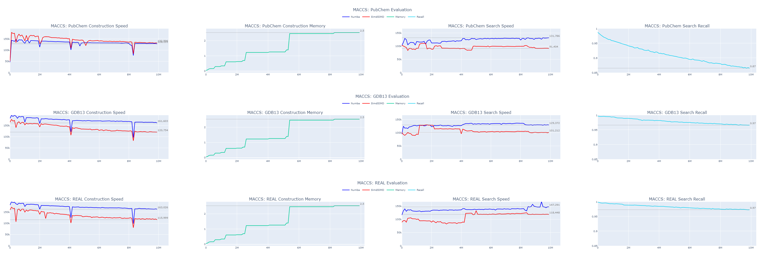
The accuracy varies between datasets. Previous observations indicate that the order in which data is indexed can significantly affect both throughput and recall, so shuffling your data when possible is advisable. In our case, we’ve used only 166 bits of the MACCS fingerprints out of a total of 5143 bits available per molecule, accounting for just 3.2% of the data. Even so, we’ve achieved 87% recall on a 10 million molecule sample from the PubChem dataset and 97% recall on samples from GDB13 and REAL.

It will continue declining as we grow the dataset. So, our next step is to enhance our accuracy.

Accuracy Improvements

Enhancing Representations with Concatenated Embeddings

One of our initial approaches was to combine multiple fingerprints into a single, more descriptive representation for each molecule. However, this meant that our existing implementation with Numba needed adjustments to handle varying lengths. Here’s how we adapted our method for vectors of an arbitrary length, ( X ):

 1
 2
 3
 4
 5
 6
 7
 8
 9
10

@cfunc(numba_signature)
def tanimoto_x(a, b):
    a_array = carray(a, x)
    b_array = carray(b, x)
    ands = 0
    ors = 0
    for i in range(x):
        ands += word_popcount(a_array[i] & b_array[i])
        ors += word_popcount(a_array[i] | b_array[i])
    return 1 - types.float32(ands) / ors

While this approach did enhance accuracy, it also increased the size of our index and resulted in a decrease in system throughput. For example, with the first 10 million molecules from the GDB 13 dataset, we observed the following metrics:

We significantly improved recall but at the cost of performance.

Implementing Conditional Similarity Metrics

To regain some performance, we employed a technique to reduce the number of bit comparisons. When working with concatenated MACCS and ECFP4 fingerprints, we first compared the MACCS section. If the similarity was below a certain threshold, only then did we proceed to compare the ECFP4 part.

 1
 2
 3
 4
 5
 6
 7
 8
 9
10
11
12
13
14
15
16
17
18
19
20
21
22
23
24
25

@cfunc(numba_signature)
def tanimoto_conditional(a, b):
    threshold = 0.2
    a_array = carray(a, 6 + 64)
    b_array = carray(b, 6 + 64)

    # Comparing MACCS prefix
    ands_maccs = 0
    ors_maccs = 0
    for i in range(6):
        ands_maccs += word_popcount(a_array[i] & b_array[i])
        ors_maccs += word_popcount(a_array[i] | b_array[i])
    maccs = 1 - types.float32(ands_maccs) / ors_maccs
    if maccs > threshold:
        return maccs

    # Comparing ECFP4 suffix
    ands_ecfp4 = 0
    ors_ecfp4 = 0
    for i in range(64):
        ands_ecfp4 += word_popcount(a_array[6 + i] & b_array[6 + i])
        ors_ecfp4 += word_popcount(a_array[6 + i] | b_array[6 + i])
    ecfp4 = 1 - types.float32(ands_ecfp4) / ors_ecfp4

    return ecfp4 * threshold

With the tanimoto_conditional metric, we managed to maintain our recall while gaining about 60% in throughput. This kept us above 100,000 queries per second across all datasets.

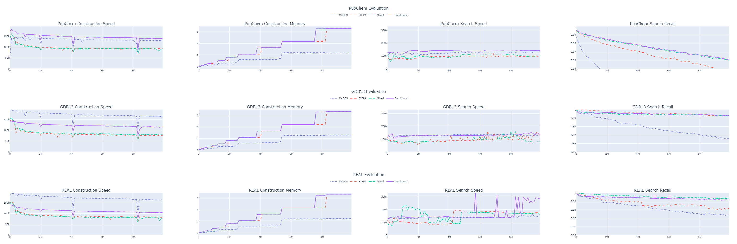
Although the 99% recall for 10 million molecules in the GDB 13 dataset is promising, we must consider this is only 1% of the entire dataset. Extrapolating, we might expect a recall of around 87% for the full billion molecules.

Fine-Tuning HNSW Hyper-Parameters

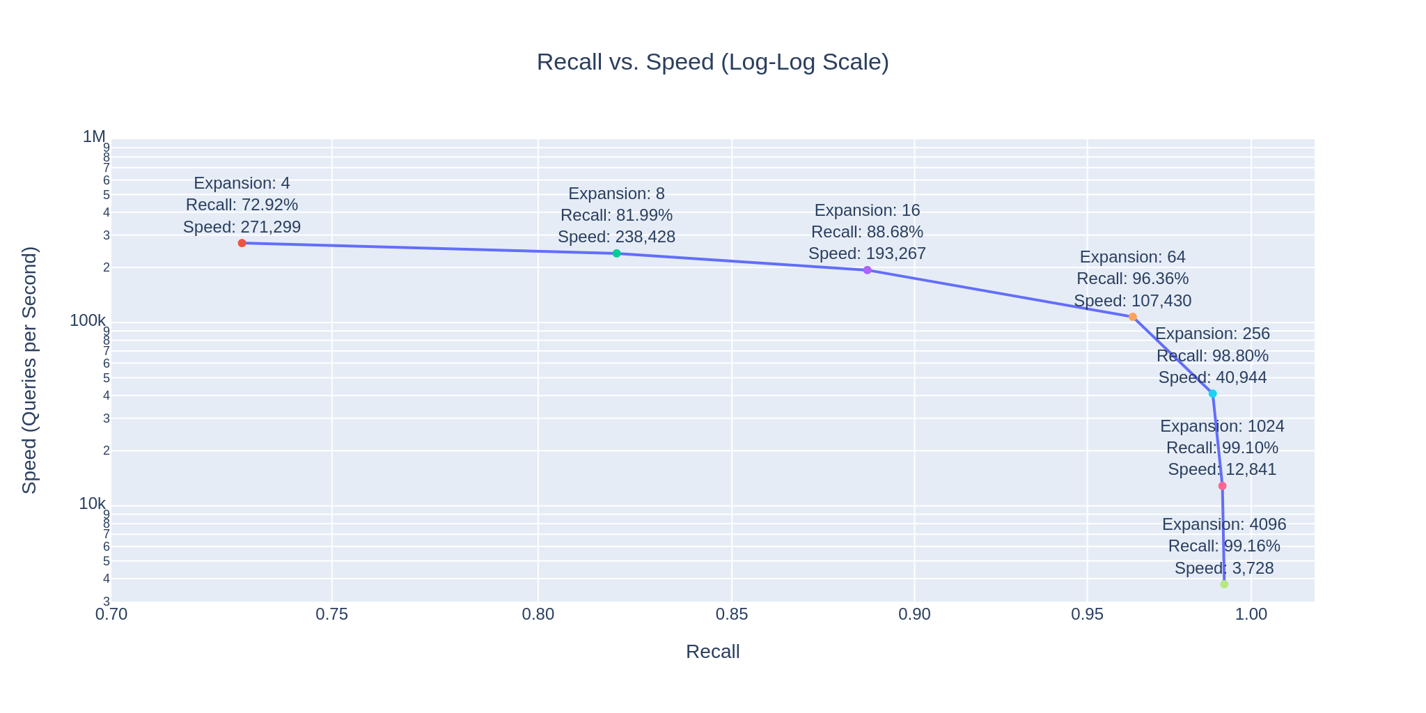
The initial step for many in data science is to tweak hyper-parameters. Our USearch Index, built on the HNSW structure, provides three key hyper-parameters: one for structure (‘connectivity’) and two for the expansion factors during ‘add’ and ‘search’ operations. The latter allows us to balance the trade-off between search speed and accuracy. The following graph shows that as expansion factors increase, accuracy improves but the speed decreases.

Comparing these numbers with brute-force search costs is insightful. Given our advanced Assembly optimizations, the cost of similarity computations is negligible. What matters is the effective memory bandwidth, which is of the order of 200 GB/s on our machine.

• Comparing only MACCS fingerprints requires fetching 21 GB of data into RAM, implying about 10 queries per second on a similar machine.
• Including ECFP4 increases the data to 277 GB, dropping the rate to approximately 1 query per second.

However, with the HNSW index, we manage an impressive 99.41% recall at 3,728 queries per second, making just 52,560 comparisons per query on average. This is just 0.005256% of our dataset, suggesting an efficiency of 99.994744%.

These numbers illustrate, how easy it is to control the tradeoff between search speed and accuracy. To visually demonstrate this, we have integrated 3Dmol.js into a StreamLit-based GUI application, available in the code repository.

In Closing

The Web is bigger than Google.

And Search is bigger than the Web.

For those who share this view, I invite you to explore our latest search benchmarks for more conventional AI-produced embeddings and keep an eye on the upcoming USearch enhancements. Plenty are coming!

Suppose you’re interested in delving into the datasets in a home setting without an HPC cluster or want to show cool-looking molecules to your kids on a laptop. In that case, we’ve placed a smaller “example” dataset in the S3 bucket for easier access and exploration. 🤗

 1
 2
 3
 4
 5
 6
 7
 8
 9
10
11

.
└── data
    └── example # 1.8 GB
        ├── index-maccs.usearch # 329 MB
        ├── index-maccs-ecfp4.usearch # 817 MB
        ├── parquet # 30 GB
        │   ├── 0000000000-0001000000.parquet # 265 MB
        │   └── 0001000000-0002000000.parquet # 265 MB
        └── smiles # 30 GB
            ├── 0000000000-0001000000.smi # 58 MB
            └── 0001000000-0002000000.smi # 58 MB