Understanding SIMD: Infinite Complexity of Trivial Problems

This blogpost is a mirror of the original post on Modular.com.

Modern CPUs have an incredible superpower: super-scalar operations, made available through single instruction, multiple data (SIMD) parallel processing. Instead of doing one operation at a time, a single core can do up to 4, 8, 16, or even 32 operations in parallel. In a way, a modern CPU is like a mini GPU, able to perform a lot of simultaneous calculations. Yet, because it’s so tricky to write parallel operations, almost all that potential remains untapped, resulting in code that only does one operation at a time

Recently, the four of us, Ash Vardanian (@ashvardanian), Evan Ovadia (@verdagon), Daniel Lemiere (@lemire), and Chris Lattner (@clattner_llvm) talked about what’s holding developers back from effectively using super-scalar operations more, and how we can create better abstractions for writing optimal software for CPUs.

Here, we share what we learned from years of implementing SIMD kernels in the SimSIMD library, which currently powers vector math in dozens of Database Management Systems (DBMS) products and AI companies–with software deployed on well over 100 million devices. While the first SIMD instruction sets were defined as early as 1966, the pain points of working with SIMD have been persistent:

High-performance computing is practically reverse-engineering of architecture details. Auto-vectorization is unreliable: the compiler can’t reliably figure this out for us. SIMD instructions are complex, and even Arm is starting to look more “CISCy” than x86! Performance is unpredictable, even for the same instruction sets shared across different CPUs. Debugging is complex: there’s no easy way to view the registers. CPU-specific code is tricky, whether it be compile-time or dynamic dispatch. Computation precision is inconsistent for floating point operations across different CPUs and instruction sets. Let’s explore these challenges and how Mojo helps address them by implementing one of the most trivial yet widespread operations in machine learning: cosine similarity. Cosine similarity computes how close two vectors are to one another by measuring the angle between the vectors.

Introduction to Cosine Similarity

You might be surprised by the widespread use of cosine similarity. Farming robots use it to zap 200,000 weeds per hour with vision-guided lasers, new ML-based methods use it for improving the speed and accuracy of climate models, and nearly every Retrieval Augmented Generation (RAG) pipeline measures the similarity of user prompts to existing knowledge bases with cosine similarity.

The following simplified diagram illustrates how RAG uses cosine similarity. A language processing ML pipeline converts text into vectors that numerically capture the meaning of words and sentences, with similar vectors sharing similar meanings. These semantically meaningful vectors are called embeddings. Cosine similarity is a way to compute the difference between embedding vectors, determining if they are semantically similar.

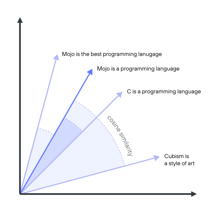
Simplified example of measuring embedding distance. Adapted from Samuel Partee

Cosine similarity can be expressed with this trivial Python code snippet, which takes the dot product of two vectors normalized by the length of the vectors:

1
2
3
4
5
6
7
8

def cosine_similarity(a: list[float], b: list[float]) -> float:
    dot_product = sum(ai * bi for ai, bi in zip(a, b))
    norm_a = sum(ai * ai for ai in a) ** 0.5
    norm_b = sum(bi * bi for bi in b) ** 0.5
    if norm_a == 0 or norm_b == 0: return 1
    if dot_product == 0: return 0
    return dot_product / (norm_a * norm_b)

Despite this algorithm’s simplicity, we can squeeze several orders of magnitude of performance out of this code. In NumPy, the same algorithm can be implemented as follows:

1
2
3
4
5
6
7
8
9

import numpy as np

def cosine_similarity(a: np.ndarray, b: np.ndarray) -> float:    
    a, b = np.asarray(a), np.asarray(b)
    dot_product = np.dot(a, b)
    norm_a, norm_b = np.linalg.norm(a), np.linalg.norm(b)
    if norm_a == 0 or norm_b == 0: return 1
    if dot_product == 0: return 0
    return dot_product / (norm_a * norm_b)

The NumPy implementation illustrates a marked improvement over the naive algorithm, but we can do even better!

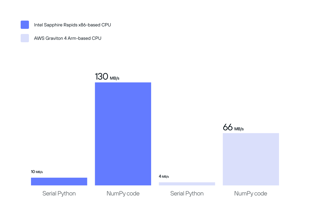
Performance of naive serial Python and NumPy implementations of cosine similarity.

In the remainder of this article, we’ll implement cosine similarity using C, taking advantage of common SIMD instructions available for various CPUs. We will also write a dispatch function that chooses different algorithms depending on our CPU. Along the way, we’ll discuss the intricacies and complexities of SIMD programming and how to solve them.

In Part 2 of this series, we’ll show how Mojo makes it easy to write similarly performant algorithms using built-in language features, so subscribe to the Modular’s RSS feed to get notified when that comes!

Mixed Precision

For the remainder of this article, we’ll be using the most common numeric type in Machine Learning these days, the bfloat16 type.

bfloat16 is a 16-bit floating point number type with a much smaller range and precision than the IEEE-standard float32 type, making it much faster to compute with. It’s also different from the IEEE-standard b type.

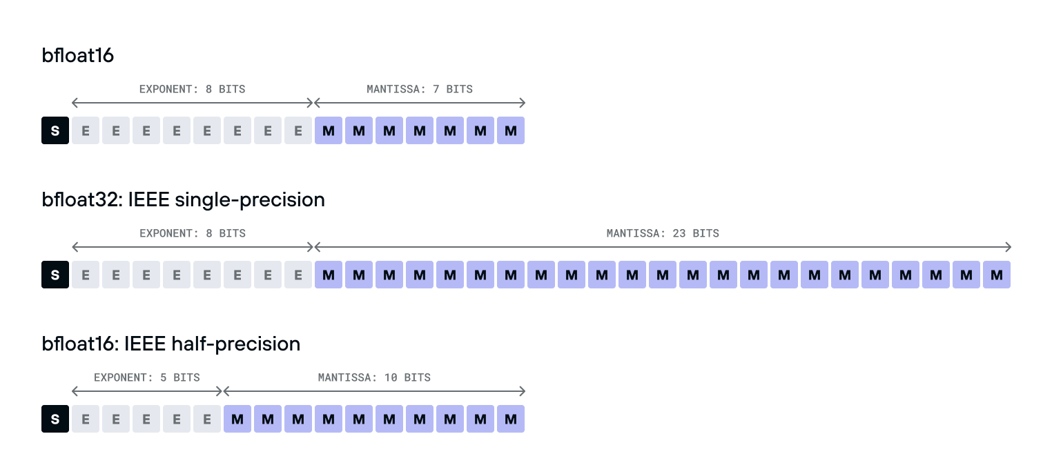
bfloat16 compared to bfloat32

Surprising to many, the bfloat16 is much easier to convert to and from float32 than float16 is - it’s just a single bit shift, because its exponent takes the same number of bits. This makes it much easier to use in practice, even on older hardware without native support: just shift to convert it to a float32, use a float32 instruction, and shift to convert it back.

But as much as we like bfloat16, we shouldn’t use it exclusively. The imprecision introduced by the type can compound quickly leading to wildly inaccurate results. To address this, we can mix different numeric types in the same computation.

For example, we could use bfloat16 for the vectors, multiply into float32 accumulators, and upcast further to float64 for the final normalization. In C++23 it would look like this:

 1
 2
 3
 4
 5
 6
 7
 8
 9
10
11
12
13
14

#include <cmath> // std::sqrt
#include <stdfloat> // std::bfloat16_t, std::float32_t, std::float64_t

std::float64_t cosine_similarity(std::bfloat16_t const * a, std::bfloat16_t const * b, std::size_t n) noexcept {
    std::float32_t dot_product = 0, norm_a = 0, norm_b = 0;
    for (std::size_t i = 0; i < n; i++) {
        std::float32_t ai = a[i], bi = b[i];
        dot_product += ai * bi, norm_a += ai * ai, norm_b += bi * bi;
    }
    if (dot_product == 0) return 0;
    if (norm_a == 0 || norm_b == 0) return 1;
    return dot_product / (std::sqrt(norm_a) * std::sqrt(norm_b));
}

Unfortunately, there are several issues with this code.

First, the C++ standard doesn’t require those types to be defined, so not every compiler will have them. Portable code with these faster data types generally requires more effort.

Second, it’s well known that even in data-parallel code like this, compilers have a hard time vectorizing low-precision code, sometimes leaving as much as 99% of single-core performance on the table, and with mixed precision it’s even worse! One needs to be explicit if they want reliable data parallelism.

Lastly, double-precision division, combined with a bit-accurate std::sqrt implementation, introduces several code branches and a lot of latency for small inputs. We can avoid these by using faster instructions.

To solve these problems, let’s use rsqrt reciprocal square root $(1/√x)$ approximations, and explicitly use SIMD intrinsics to accelerate this code for every common target platform.

Let’s start by looking at some C 99 cross-platform kernels from my SimSIMD library.

Baseline implementation for Intel Haswell

Intel Haswell and newer generations of x86 CPUs all support AVX2, which is a 256-bit SIMD instruction set for the 32 new YMM register files on the CPU. This allows us to do 8 simultaneous float32 operations at a time.

Here’s roughly what our above kernel would look like, specialized for AVX2 hardware.

 1
 2
 3
 4
 5
 6
 7
 8
 9
10
11
12
13
14
15
16
17
18
19
20
21
22

void simsimd_cos_bf16_haswell(simsimd_bf16_t const * a, simsimd_bf16_t const * b, simsimd_size_t n, simsimd_distance_t * result) {
    __m256 a_vec, b_vec;
    // Initialize our accumulators, each will have 8 words/scalars.
    __m256 ab_vec = _mm256_setzero_ps(), a2_vec = _mm256_setzero_ps(), b2_vec = _mm256_setzero_ps();

    while (n) {
        // Load the next 128 bits from the inputs, then cast.
        a_vec = _simsimd_bf16x8_to_f32x8_haswell(_mm_loadu_si128((__m128i const*)a));
        b_vec = _simsimd_bf16x8_to_f32x8_haswell(_mm_loadu_si128((__m128i const*)b));
        n -= 8, a += 8, b += 8;
        // TODO: Handle input lengths that aren't a multiple of 8

        // Multiply and add them to the accumulator variables.
        ab_vec = _mm256_fmadd_ps(a_vec, b_vec, ab_vec);
        a2_vec = _mm256_fmadd_ps(a_vec, a_vec, a2_vec);
        b2_vec = _mm256_fmadd_ps(b_vec, b_vec, b2_vec);
    }

    // TODO: Reduce; combine the 8 words/scalars into one scalar number.
    // TODO: Normalize and divide, like: *result = ab / (sqrt(a2) * sqrt(b2))
}

We’ll implement the TODO blocks later below, but you can also see the completed simsimd_cos_bf16_haswell implementation in simsimd/spatial.h.

This loop does three main things.

First, it uses _mm_loadu_si128 to load 128 bits from a potentially unaligned memory address. One should be careful to use this instead of _mm_load_si128 which crashes if the address of the vector is not divisible by 16, which is the XMM register size in bytes.

Second, it uses _simsimd_bf16x8_to_f32x8_haswell to convert from bfloat16 to float32. It interprets the input as 8 16-bit integers and converts them to 32-bit integers, and then shift them left by 16 bits:

1
2
3

__m256 _simsimd_bf16x8_to_f32x8_haswell(__m128i a) {
    return _mm256_castsi256_ps(_mm256_slli_epi32(_mm256_cvtepu16_epi32(a), 16));
}

Third, we use _mm256_fmadd_ps to accumulate our dot product into ab_vec’s 8 scalars by multiplying a_vec’s 8 words with b_vec’s 8 words. This is a fused multiply-add (FMA) instruction, which is faster than multiplying and adding numbers individually:

For most of those instructions and CPU core designs, two such operations can be performed simultaneously. We call FMA three times in each cycle. Once for the actual dot product and twice to accumulate “squared norms” into a2_vec and b2_vec.

After the loop, we’ll need to horizontally accumulate, which means add the 8 words of ab_vec together to get one single number. Let’s talk about how!

Reducing Horizontal Accumulations

A tricky part of SIMD in practice is to avoid horizontal accumulation of the entire register, because it’s a slow operation.

Whenever possible, accumulation should be placed outside of the loop, which generally requires some intra-register shuffling for a tree-like reduction.

For example, _simsimd_reduce_f32x8_haswell may look like this under the hood:

 1
 2
 3
 4
 5
 6
 7
 8
 9
10
11
12

simsimd_f64_t _simsimd_reduce_f32x8_haswell(__m256 vec) {
    __m128 low_f32 = _mm256_castps256_ps128(vec);
    __m128 high_f32 = _mm256_extractf128_ps(vec, 1);
    __m256d low_f64 = _mm256_cvtps_pd(low_f32);
    __m256d high_f64 = _mm256_cvtps_pd(high_f32);
    __m256d sum = _mm256_add_pd(low_f64, high_f64);
    __m128d sum_low = _mm256_castpd256_pd128(sum);
    __m128d sum_high = _mm256_extractf128_pd(sum, 1);
    __m128d sum128 = _mm_add_pd(sum_low, sum_high);
    sum128 = _mm_hadd_pd(sum128, sum128);
    return _mm_cvtsd_f64(sum128);
}

In our function, we’ll use it like this:

1
2
3

simsimd_f64_t ab = _simsimd_reduce_f32x8_haswell(ab_vec);
simsimd_f64_t a2 = _simsimd_reduce_f32x8_haswell(a2_vec);
simsimd_f64_t b2 = _simsimd_reduce_f32x8_haswell(b2_vec);

Now, we have:

• A single ab number, the dot product of a and b.
• A single a2 number, the dot product of a with itself, the “squared norm” of a.
• A similar squared norm of b.

Reciprocal square root approximation in AVX2

Our function’s last line will be this:

1

*result = _simsimd_cos_normalize_f64_haswell(ab, a2, b2);

It will need to do the dot product of a and b, divided by the normalized a and the normalized b, like this pseudocode:

1

*result = ab / (sqrt(a2) * sqrt(b2))

That’s right: to normalize the result, not one, but two square roots are required.

We’ll use the _mm_rsqrt_ps instruction. It’s not available for double-precision floats, but it’s still a great choice for single-precision floats. Our function would look something like this:

 1
 2
 3
 4
 5
 6
 7
 8
 9
10
11
12
13
14

simsimd_distance_t _simsimd_cos_normalize_f64_haswell(simsimd_f64_t ab, simsimd_f64_t a2, simsimd_f64_t b2) {
    if (ab == 0) return 0;
    if (a2 == 0 || b2 == 0) return 1;

    __m128d squares = _mm_set_pd(a2, b2);
    __m128d rsqrts = _mm_cvtps_pd(_mm_rsqrt_ps(_mm_cvtpd_ps(squares)));
    
    // TODO: More precision!

    simsimd_f64_t a2_reciprocal = _mm_cvtsd_f64(_mm_unpackhi_pd(rsqrts, rsqrts));
    simsimd_f64_t b2_reciprocal = _mm_cvtsd_f64(rsqrts);
    return ab * a2_reciprocal * b2_reciprocal;
}

However, the _mm_rsqrt_ps instruction can introduce errors as high as 1.5*2^-12, as documented by Intel.

A great 2009 article Timing Square Root comparing the accuracy and speed of the native rsqrt instruction (present in SSE and newer x86 SIMD instruction sets) with John Carmack’s fast inverse square root mentions using a Newton-Raphson iteration as an alternative to improve numerical accuracy, and we’ll do something similar here to improve our algorithm:

 1
 2
 3
 4
 5
 6
 7
 8
 9
10
11
12
13
14
15
16

simsimd_distance_t _simsimd_cos_normalize_f64_haswell(simsimd_f64_t ab, simsimd_f64_t a2, simsimd_f64_t b2) {
    if (ab == 0) return 0;
    if (a2 == 0 || b2 == 0) return 1;

    __m128d squares = _mm_set_pd(a2, b2);
    __m128d rsqrts = _mm_cvtps_pd(_mm_rsqrt_ps(_mm_cvtpd_ps(squares)));
    
    // Newton-Raphson iteration:
    rsqrts = _mm_add_pd(
        _mm_mul_pd(_mm_set1_pd(1.5), rsqrts),
        _mm_mul_pd(_mm_mul_pd(_mm_mul_pd(squares, _mm_set1_pd(-0.5)), rsqrts), _mm_mul_pd(rsqrts, rsqrts)));

    simsimd_f64_t a2_reciprocal = _mm_cvtsd_f64(_mm_unpackhi_pd(rsqrts, rsqrts));
    simsimd_f64_t b2_reciprocal = _mm_cvtsd_f64(rsqrts);
    return ab * a2_reciprocal * b2_reciprocal;
}

One must keep in mind, various CPUs’ rsqrt instructions will have different performance and accuracy. After we finish our simsimd_cos_bf16_haswell function, we’ll see how this compares to AVX-512 further below.

Partial Loads

There’s still an assumption we have to fix, inside our loop:

1

// TODO: Handle input lengths that aren't a multiple of 8

Potentially the ugliest part of this and many other production SIMD codebases is the “partial load” logic.

It’s a natural consequence of slicing variable-length data into fixed-register-length chunks.

Because of this, almost every kernel has the “main loop” and a “tail loop” for the last few elements.

Prior to AVX-512 on x86 and SVE on Arm, there was no way to load a partial register, so the code has to be a bit more complex.

In Part 2, we’ll talk about how Mojo solves this problem. But for now, we’ll handle it manually by adding this inside the loop:

1
2
3
4
5
6

    if (n < 8) {
        a_vec = _simsimd_bf16x8_to_f32x8_haswell(_simsimd_partial_load_bf16x8_haswell(a, n));
        b_vec = _simsimd_bf16x8_to_f32x8_haswell(_simsimd_partial_load_bf16x8_haswell(b, n));
        n = 0;
    } else {
        ...

That’s it! Here’s the complete function below. And as a bonus, we changed the while loop to a goto because that’s just how I roll. Oftentimes, goto usage is discouraged in modern codebases, but in small functions they don’t convolute the control flow and can help reason about code in a more machine-accurate way. CPU’s don’t have for loops after all. Moreover, this way we avoid code duplication for the primary logic instead of repeating it twice in the main loop and the tail.

 1
 2
 3
 4
 5
 6
 7
 8
 9
10
11
12
13
14
15
16
17
18
19
20
21
22
23
24
25

void simsimd_cos_bf16_haswell(simsimd_bf16_t const * a, simsimd_bf16_t const * b, simsimd_size_t n, simsimd_distance_t * result) {
    __m256 a_vec, b_vec;
    __m256 ab_vec = _mm256_setzero_ps(), a2_vec = _mm256_setzero_ps(), b2_vec = _mm256_setzero_ps();

simsimd_cos_bf16_haswell_cycle:
    if (n < 8) {
        a_vec = _simsimd_bf16x8_to_f32x8_haswell(_simsimd_partial_load_bf16x8_haswell(a, n));
        b_vec = _simsimd_bf16x8_to_f32x8_haswell(_simsimd_partial_load_bf16x8_haswell(b, n));
        n = 0;
    } else {
        a_vec = _simsimd_bf16x8_to_f32x8_haswell(_mm_loadu_si128((__m128i const*)a));
        b_vec = _simsimd_bf16x8_to_f32x8_haswell(_mm_loadu_si128((__m128i const*)b));
        n -= 8, a += 8, b += 8;
    }
    ab_vec = _mm256_fmadd_ps(a_vec, b_vec, ab_vec);
    a2_vec = _mm256_fmadd_ps(a_vec, a_vec, a2_vec);
    b2_vec = _mm256_fmadd_ps(b_vec, b_vec, b2_vec);
    if (n)
        goto simsimd_cos_bf16_haswell_cycle;

    simsimd_f64_t ab = _simsimd_reduce_f32x8_haswell(ab_vec);
    simsimd_f64_t a2 = _simsimd_reduce_f32x8_haswell(a2_vec);
    simsimd_f64_t b2 = _simsimd_reduce_f32x8_haswell(b2_vec);
    *result = _simsimd_cos_normalize_f64_haswell(ab, a2, b2);
}

You can also see simsimd_cos_bf16_haswell live, in simsimd/spatial.h.

Now we are done with one of the most “vanilla” kernels in SimSIMD. It targets broadly available CPUs starting with Intel Haswell, shipped from 2013 onwards. It is forward-compatible with 11 years of x86 hardware, performing mixed-precision operations in bf16-f32-f64, including numeric types not natively supported by hardware. This is a good warmup, but the most exciting parts of SimSIMD, and the reason it runs on hundreds of millions of devices, are still ahead!

Baseline implementation for AMD Genoa

Let’s kick it up a notch, and bring in AVX-512, which is a 512-bit SIMD instruction set for the 32 new ZMM register files on the CPU. AMD Genoa is the first AMD CPU to support it, and it’s also the earliest publicly available CPU with AVX512_BF16 “extension of extension” for the bfloat16 type, including the vdpbf16ps instruction for dot products.

Before we show the masking and the vdpbf16ps parts, here’s roughly what our simsimd_cos_bf16_genoa will look like:

 1
 2
 3
 4
 5
 6
 7
 8
 9
10
11
12
13
14
15
16
17
18
19
20
21
22
23
24
25
26
27
28
29

void simsimd_cos_bf16_genoa(
    simsimd_bf16_t const * a, simsimd_bf16_t const * b,
    simsimd_size_t n,
    simsimd_distance_t * result) {

    __m512 ab_vec = _mm512_setzero_ps();
    __m512 a2_vec = _mm512_setzero_ps();
    __m512 b2_vec = _mm512_setzero_ps();
    __m512i a_i16_vec, b_i16_vec;

simsimd_cos_bf16_genoa_cycle:
    if (n < 32) {
        // TODO: Partial ("masked") load from a and b.
        n = 0;
    } else {
        a_i16_vec = _mm512_loadu_epi16(a);
        b_i16_vec = _mm512_loadu_epi16(b);
        a += 32, b += 32, n -= 32;
    }
    // TODO: Add to ab_vec/a2_vec/b2_vec with special dot-product instruction.

    if (n)
        goto simsimd_cos_bf16_genoa_cycle;

    simsimd_f64_t ab = _simsimd_reduce_f32x16_skylake(ab_vec);
    simsimd_f64_t a2 = _simsimd_reduce_f32x16_skylake(a2_vec);
    simsimd_f64_t b2 = _simsimd_reduce_f32x16_skylake(b2_vec);
    *result = _simsimd_cos_normalize_f64_skylake(ab, a2, b2);
}

Structurally, the kernel is similar, but the loop step size grew from 8 to 32, and even bigger changes are hiding behind those TODOs.

You may have noticed that a_i16_vec and b_i16_vec are represented with __m512i, as opposed to the bfloat16 vector type __m512bh. This is caused by incomplete support for loadu intrinsics, missing a bfloat16 overload in some compilers.

Now, let’s resolve those TODOs, starting with the masked loads.

Masking in x86 AVX-512

AVX-512 was the first SIMD instruction set to introduce masking, which is a way to partially execute instructions based on a mask. For example, if you have a register containing 8 words/scalars, you can use a mask to increment only 5 of them.

Each core contains not only 32 ZMM registers, but also 8 KMASK registers, which can be used to control the execution of instructions. Think of them as 8 additional normal scalar registers, containing 8, 16, 32, or 64 bits. Moving between those and general-purpose registers isn’t free, but using them for masking is still better than branching.

Interleaving, testing, and merging masks with each other is also natively supported with these special mask manipulation instructions:

 1
 2
 3
 4
 5
 6
 7
 8
 9
10
11
12

int _mm512_kortestc(__mmask16 k1, __mmask16 k2);        // `kortestw`
int _mm512_kortestz(__mmask16 k1, __mmask16 k2);        // `kortestw`
__mmask16 _mm512_kand(__mmask16 a, __mmask16 b);        // `kandw`
__mmask16 _mm512_kandn(__mmask16 a, __mmask16 b);       // `kandnw`
__mmask16 _mm512_kmov(__mmask16 a);                     // `kmovw`
__mmask16 _mm512_knot(__mmask16 a);                     // `knotw`
__mmask16 _mm512_kor(__mmask16 a, __mmask16 b);         // `korw`
__mmask16 _mm512_kunpackb(__mmask16 a, __mmask16 b);    // `kunpckbw`
__mmask16 _mm512_kxnor(__mmask16 a, __mmask16 b);       // `kxnorw`
__mmask16 _mm512_kxor(__mmask16 a, __mmask16 b);        // `kxorw`
__mmask32 _mm512_kunpackw(__mmask32 a, __mmask32 b);    // `kunpckwd`
__mmask64 _mm512_kunpackd(__mmask64 a, __mmask64 b);    // `kunpckdq`

When using SIMD, it can be easy to accidentally load past the end of the array, since we’re loading in chunks, and the array might not be a multiple of our vector size. To avoid that, we’ll do some masking to partially load from a and b in the last iteration. Our if-else looks like this now:

 1
 2
 3
 4
 5
 6
 7
 8
 9
10

if (n < 32) {
    __mmask32 mask = (__mmask32)_bzhi_u32(0xFFFFFFFF, n);
    a_i16_vec = _mm512_maskz_loadu_epi16(mask, a);
    b_i16_vec = _mm512_maskz_loadu_epi16(mask, b);
    n = 0;
} else {
    a_i16_vec = _mm512_loadu_epi16(a);
    b_i16_vec = _mm512_loadu_epi16(b);
    a += 32, b += 32, n -= 32;
}

Dot Products with vdpbf16ps

Let’s resolve this TODO now:

1

// TODO: Add to ab_vec/a2_vec/b2_vec with special dot-product instruction.

Previously, in our simsimd_cos_bf16_haswell kernel, we added 8 input bfloat16s to ab_vec etc. with this code:

1
2
3

ab_vec = _mm256_fmadd_ps(a_vec, b_vec, ab_vec);
a2_vec = _mm256_fmadd_ps(a_vec, a_vec, a2_vec);
b2_vec = _mm256_fmadd_ps(b_vec, b_vec, b2_vec);

ab_vec is 512 bits wide, and holds 16 float32s. You might think that we would now add 16 input bfloat16s to it, but it’s even better than that: the vdpbf16ps processes 32 input numbers into our 16-word ab_vec. It takes the dot product of the first two words of each input, and add their dot-products to the first word of the result (like ab_vec[0] += a[0] * b[0] + a[1] * b[1]), and then it does that for the rest of the words as well.

We’ll use the _mm512_dpbf16_ps function to do this instruction, and add this to our loop:

1
2
3

ab_vec = _mm512_dpbf16_ps(ab_vec, (__m512bh)(a_i16_vec), (__m512bh)(b_i16_vec));
a2_vec = _mm512_dpbf16_ps(a2_vec, (__m512bh)(a_i16_vec), (__m512bh)(a_i16_vec));
b2_vec = _mm512_dpbf16_ps(b2_vec, (__m512bh)(b_i16_vec), (__m512bh)(b_i16_vec));

Here’s the full function:

 1
 2
 3
 4
 5
 6
 7
 8
 9
10
11
12
13
14
15
16
17
18
19
20
21
22
23
24
25
26
27
28
29

void simsimd_cos_bf16_genoa(
    simsimd_bf16_t const * a, simsimd_bf16_t const * b,
    simsimd_size_t n,
    simsimd_distance_t * result) {
    __m512 ab_vec = _mm512_setzero_ps();
    __m512 a2_vec = _mm512_setzero_ps();
    __m512 b2_vec = _mm512_setzero_ps();
    __m512i a_i16_vec, b_i16_vec;
simsimd_cos_bf16_genoa_cycle:
    if (n < 32) {
        __mmask32 mask = (__mmask32)_bzhi_u32(0xFFFFFFFF, n);
        a_i16_vec = _mm512_maskz_loadu_epi16(mask, a);
        b_i16_vec = _mm512_maskz_loadu_epi16(mask, b);
        n = 0;
    } else {
        a_i16_vec = _mm512_loadu_epi16(a);
        b_i16_vec = _mm512_loadu_epi16(b);
        a += 32, b += 32, n -= 32;
    }
    ab_vec = _mm512_dpbf16_ps(ab_vec, (__m512bh)(a_i16_vec), (__m512bh)(b_i16_vec));
    a2_vec = _mm512_dpbf16_ps(a2_vec, (__m512bh)(a_i16_vec), (__m512bh)(a_i16_vec));
    b2_vec = _mm512_dpbf16_ps(b2_vec, (__m512bh)(b_i16_vec), (__m512bh)(b_i16_vec));
    if (n)
        goto simsimd_cos_bf16_genoa_cycle;
    simsimd_f64_t ab = _simsimd_reduce_f32x16_skylake(ab_vec);
    simsimd_f64_t a2 = _simsimd_reduce_f32x16_skylake(a2_vec);
    simsimd_f64_t b2 = _simsimd_reduce_f32x16_skylake(b2_vec);
    *result = _simsimd_cos_normalize_f64_skylake(ab, a2, b2);
}

Now let’s implement that _simsimd_cos_normalize_f64_skylake call at the end!

Reciprocal square root approximation for AVX-512

We need to conceptually calculate ab / (sqrt(a2) * sqrt(b2)).

In our _simsimd_cos_normalize_f64_haswell function from before, we used the rsqrtps instruction (via the _mm_rsqrt_ps intrinsic) to calculate our reciprocal square root. In AVX-512, those are superseded by the _mm512_rsqrt14_ps intrinsic and vrsqrt14ps instruction.

And fortunately, the maximum error bound improved from 1.5*2^-12 to 2^-14.

There is also a double-precision instruction vrsqrt14pd (via the _mm512_rsqrt14_pd intrinsic).

It has the same precision, but we can avoid casting.

 1
 2
 3
 4
 5
 6
 7
 8
 9
10
11
12
13
14

simsimd_distance_t _simsimd_cos_normalize_f64_skylake(simsimd_f64_t ab, simsimd_f64_t a2, simsimd_f64_t b2) {
    if (ab == 0) return 0;
    if (a2 == 0 || b2 == 0) return 1;

    __m128d squares = _mm_set_pd(a2, b2);
    __m128d rsqrts = _mm_maskz_rsqrt14_pd(0xFF, squares);
    rsqrts = _mm_add_pd( // Newton-Raphson iteration:
        _mm_mul_pd(_mm_set1_pd(1.5), rsqrts),
        _mm_mul_pd(_mm_mul_pd(_mm_mul_pd(squares, _mm_set1_pd(-0.5)), rsqrts), _mm_mul_pd(rsqrts, rsqrts)));

    simsimd_f64_t a2_reciprocal = _mm_cvtsd_f64(_mm_unpackhi_pd(rsqrts, rsqrts));
    simsimd_f64_t b2_reciprocal = _mm_cvtsd_f64(rsqrts);
    return ab * a2_reciprocal * b2_reciprocal;
}

A natural question may be: how important is this Newton-Raphson iteration?

As you can see, it reduces our relative error by a lot. On 1536-dimensional inputs, the impact is as big as 2-3 orders of magnitude!

Keep this impact in mind. In a little bit, we’ll see the error rate for Arm NEON’s rsqrt instruction, and just how necessary it is to stay on top of our floating point precision for specific CPUs.

This is also why abstraction can be difficult and/or counterproductive when dealing with SIMD. The entire shape of the algorithm (such as whether we do a Newton-Raphson iteration) can change depending on the CPU or the precision of its instructions.

Baseline implementation for Arm NEON

Most CPUs aren’t running x86, but Arm. Apple alone today accounts for 2.2 billion devices, and almost all of them run on Arm. Arm devices also have a SIMD instruction set, called NEON, which is similar to SSE, also with 128-bit registers.

 1
 2
 3
 4
 5
 6
 7
 8
 9
10
11
12
13
14
15
16
17
18
19
20
21
22
23
24
25
26
27
28
29
30
31
32
33

void simsimd_cos_bf16_neon(
    simsimd_bf16_t const * a, simsimd_bf16_t const * b,
    simsimd_size_t n, simsimd_distance_t * result) {

    float32x4_t ab_high_vec = vdupq_n_f32(0), ab_low_vec = vdupq_n_f32(0);
    float32x4_t a2_high_vec = vdupq_n_f32(0), a2_low_vec = vdupq_n_f32(0);
    float32x4_t b2_high_vec = vdupq_n_f32(0), b2_low_vec = vdupq_n_f32(0);
    bfloat16x8_t a_vec, b_vec;

simsimd_cos_bf16_neon_cycle:
    if (n < 8) {
        a_vec = _simsimd_partial_load_bf16x8_neon(a, n);
        b_vec = _simsimd_partial_load_bf16x8_neon(b, n);
        n = 0;
    } else {
        a_vec = vld1q_bf16((bfloat16_t const*)a);
        b_vec = vld1q_bf16((bfloat16_t const*)b);
        n -= 8, a += 8, b += 8;
    }
    ab_high_vec = vbfmlaltq_f32(ab_high_vec, a_vec, b_vec);
    ab_low_vec = vbfmlalbq_f32(ab_low_vec, a_vec, b_vec);
    a2_high_vec = vbfmlaltq_f32(a2_high_vec, a_vec, a_vec);
    a2_low_vec = vbfmlalbq_f32(a2_low_vec, a_vec, a_vec);
    b2_high_vec = vbfmlaltq_f32(b2_high_vec, b_vec, b_vec);
    b2_low_vec = vbfmlalbq_f32(b2_low_vec, b_vec, b_vec);
    if (n)
        goto simsimd_cos_bf16_neon_cycle;

    simsimd_f32_t ab = vaddvq_f32(vaddq_f32(ab_high_vec, ab_low_vec)),
                  a2 = vaddvq_f32(vaddq_f32(a2_high_vec, a2_low_vec)),
                  b2 = vaddvq_f32(vaddq_f32(b2_high_vec, b2_low_vec));
    *result = _simsimd_cos_normalize_f64_neon(ab, a2, b2);
}

You may be wondering, what happened to our ab_vec, and what are these ab_high_vec and ab_low_vec things?

These, my friends, are a perfect example of my next point.

CISC vs RISC, it’s not what people say

The Arm instruction set is often called RISC (Reduced Instruction Set Computer), and the x86 instruction set is often called CISC (Complex Instruction Set Computer).

But in practice, the Arm instruction set is potentially more complex, especially given that all of those instructions practically apply only to 64-bit and 128-bit registers, as opposed to the x86 instructions which also include 256-bit and 512-bit registers!

Here is an example.

Before discovering the vbfdotq_f32 intrinsic (suggested by Mark Reed), SimSIMD used the vbfmmlaq_f32 and vbfmmlaq_f32 intrinsics to compute the dot product of two vectors.

It’s also a Fused Multiply-Add instruction, but designed to take only odd or even components of the vectors, so we aggregate them differently:

1
2
3
4
5
6

ab_high_vec = vbfmlaltq_f32(ab_high_vec, a_vec, b_vec);
ab_low_vec = vbfmlalbq_f32(ab_low_vec, a_vec, b_vec);
a2_high_vec = vbfmlaltq_f32(a2_high_vec, a_vec, a_vec);
a2_low_vec = vbfmlalbq_f32(a2_low_vec, a_vec, a_vec);
b2_high_vec = vbfmlaltq_f32(b2_high_vec, b_vec, b_vec);
b2_low_vec = vbfmlalbq_f32(b2_low_vec, b_vec, b_vec);

In other words, ab_high_vec contains only the even components, and ab_low_vec contains only the odd components.

This instruction probably makes more sense for complex dot-products, where we might want to load only the real words or only the imaginary words from a vector of complex numbers.

As for the cosine distance, there is one more non-obvious approach previously tested in SimSIMD.

NEON contains a BFMMLA instruction:

BFloat16 floating-point matrix multiply-accumulates into 2x2 matrix. This instruction multiplies the 2x4 matrix of BF16 values held in the first 128-bit source vector by the 4x2 BF16 matrix in the second 128-bit source vector. The resulting 2x2 single-precision matrix product is then added destructively to the 2x2 single-precision matrix in the 128-bit destination vector. This is equivalent to performing a 4-way dot product per destination element. The instruction ignores the FPCR and does not update the FPSR exception status.

Doesn’t look very RISCy to me! But at some point, it looked promising. Concatenating vectors $a$ and $b$ into a matrix $X$ and computing the dot product $XᵀX$ in a single instruction is a great idea. It will contain 4 dot products, and we can drop 1 of them, keeping 3 products: $ab$, $aa$, and $bb$, all needed for cosine similarity. That kernel may look similar to this:

 1
 2
 3
 4
 5
 6
 7
 8
 9
10
11
12
13
14
15
16
17
18
19
20
21

float32x4_t products_low_vec = vdupq_n_f32(0.0f);
float32x4_t products_high_vec = vdupq_n_f32(0.0f);
for (; i + 8 <= n; i += 8) {
    bfloat16x8_t a_vec = vld1q_bf16((bfloat16_t const*)a + i);
    bfloat16x8_t b_vec = vld1q_bf16((bfloat16_t const*)b + i);
    int16x8_t a_vec_s16 = vreinterpretq_s16_bf16(a_vec);
    int16x8_t b_vec_s16 = vreinterpretq_s16_bf16(b_vec);
    int16x8x2_t y_w_vecs_s16 = vzipq_s16(a_vec_s16, b_vec_s16);
    bfloat16x8_t y_vec = vreinterpretq_bf16_s16(y_w_vecs_s16.val[0]);
    bfloat16x8_t w_vec = vreinterpretq_bf16_s16(y_w_vecs_s16.val[1]);
    bfloat16x4_t a_low = vget_low_bf16(a_vec);
    bfloat16x4_t b_low = vget_low_bf16(b_vec);
    bfloat16x4_t a_high = vget_high_bf16(a_vec);
    bfloat16x4_t b_high = vget_high_bf16(b_vec);
    bfloat16x8_t x_vec = vcombine_bf16(a_low, b_low);
    bfloat16x8_t v_vec = vcombine_bf16(a_high, b_high);
    products_low_vec = vbfmmlaq_f32(products_low_vec, x_vec, y_vec);
    products_high_vec = vbfmmlaq_f32(products_high_vec, v_vec, w_vec);
}
float32x4_t products_vec = vaddq_f32(products_high_vec, products_low_vec);
simsimd_f32_t a2 = products_vec[0], ab = products_vec[1], b2 = products_vec[3];

Unfortunately, this approach ended up being 25% slower than the naive approach.

When dealing with x86 ISA, if you find a weird rare instruction that can be used in your program, it’s often a good idea to apply it.

In Arm it doesn’t help most of the time, so in my opinion, Arm is more CISCy than x86.

This is also why it’s important to have CPU-specific code, rather than relying on coarse abstractions that just use whatever instruction is present.

Reverse engineering Arm accuracy

Similar to x86, the rsqrt instruction is available in NEON, but only for single-precision floats.

Unlike x86, the documentation is limited:

1. We can’t know the latency of the instruction.
2. We are not even informed of the maximum relative error.

The first can be vaguely justified by the fact that Arm doesn’t produce its chips, it licenses the designs to other companies. Still, a repository of timings for different chips would be very helpful. Second is just a mystery. Until you reverse engineer it!

I wrote this benchmark program, which estimates the accuracy of rsqrt approximations in Arm NEON, SSE, AVX2, and AVX-512.

Luckily, it’s only 4 billion unique inputs to test, just a few seconds on a modern CPU.

Baseline implementation for Arm SVE

Arm SVE is unusual.

It’s not the first to support masking, like AVX-512.

But it is the first to define variable-width implementation-defined registers, which can be 128, 256, 512, 1024, or 2048 bits wide.

That means that on one CPU, a svbfloat16_t might be 128 bits wide (8 bfloat16s) and on another CPU it might be 1024 bits wide (fitting 64 bfloat16s), yet the compiled program is the same. One can only know their width at run-time by calling the svcnth function, which tells us how many 16-bit words fit in a SVE vector on this CPU.

At the end of this spectrum (2048 bits) the CPUs are practically converging with GPUs, but despite that, all real implementations are 128-bit wide.

This is what a kernel may look like:

 1
 2
 3
 4
 5
 6
 7
 8
 9
10
11
12
13
14
15
16
17
18
19
20
21
22
23
24
25

void simsimd_cos_bf16_sve(
    simsimd_bf16_t const* a_enum, simsimd_bf16_t const* b_enum,
    simsimd_size_t n, simsimd_distance_t* result) {

    simsimd_size_t i = 0;
    svfloat32_t ab_vec = svdupq_n_f32(0.f, 0.f, 0.f, 0.f);
    svfloat32_t a2_vec = svdupq_n_f32(0.f, 0.f, 0.f, 0.f);
    svfloat32_t b2_vec = svdupq_n_f32(0.f, 0.f, 0.f, 0.f);
    bfloat16_t const* a = (bfloat16_t const*)(a_enum);
    bfloat16_t const* b = (bfloat16_t const*)(b_enum);
    do {
        svbool_t progress_vec = svwhilelt_b16((unsigned int)i, (unsigned int)n);
        svbfloat16_t a_vec = svld1_bf16(progress_vec, a + i);
        svbfloat16_t b_vec = svld1_bf16(progress_vec, b + i);
        ab_vec = svbfdot_f32(ab_vec, a_vec, b_vec);
        a2_vec = svbfdot_f32(a2_vec, a_vec, a_vec);
        b2_vec = svbfdot_f32(b2_vec, b_vec, b_vec);
        i += svcnth();
    } while (i < n);

    simsimd_f32_t ab = svaddv_f32(svptrue_b32(), ab_vec);
    simsimd_f32_t a2 = svaddv_f32(svptrue_b32(), a2_vec);
    simsimd_f32_t b2 = svaddv_f32(svptrue_b32(), b2_vec);
    *result = _simsimd_cos_normalize_f32_neon(ab, a2, b2);
}

This is another reason it’s important to have CPU-specific code, and to not rely too heavily on abstractions: some architectures are very unusual.

Masking in Arm SVE

Seeing “variable-width implementation-defined registers” you may ask yourself, how does the final iteration of the loop handle the remainder of the elements, if they don’t fill up an entire vector? In SVE, the recommended approach is to use “progress masks” (like that progress_vec) and build them using “while less than” intrinsics (like that svwhilelt_b16). It’s a more powerful alternative to _bzhi_u32 that we’ve used for AVX-512 tails.

Adding up the performance gains

Taking a look back at all of the hardware-specific optimizations, we can see an orders-of-magnitude improvement over our initial naive implementation and stock NumPy implementation. Utilizing and exploiting hardware features has delivered performance boosts:

• from 10 MB/s to 60.3 GB/s on Intel hardware,
• and 4 MB/s to 29.7 GB/s on Arm hardware.

It underscores the absolute importance that specialized hardware acceleration libraries have on even the simplest of computational algorithms.

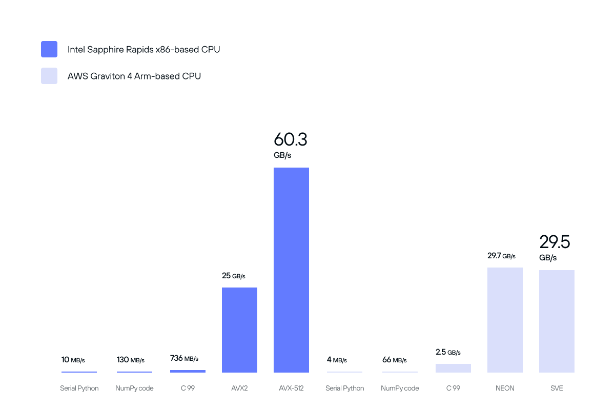
Performance improvements from architecture-specific SIMD optimizations for cosine similarity.

Packaging and distributing libraries

Throughout this post, I’ve mentioned a few times that CPU-specific code is important. But shipping CPU-specific code correctly can be tricky.

The easiest and fastest approach is just to compile for a specific hardware platform. With -march=native, for example, your compiler will compile the code assuming the target machine that will run this software supports all the same Assembly instructions as this one. We can implement several kernels for different platforms and select the best backend at compile time.

 1
 2
 3
 4
 5
 6
 7
 8
 9
10
11
12
13
14
15

void simsimd_cos_bf16(
simsimd_bf16_t const* a, simsimd_bf16_t const* b, simsimd_size_t n,
             simsimd_distance_t* d) {
#if SIMSIMD_TARGET_GENOA
    simsimd_cos_bf16_genoa(a, b, n, d);
#elif SIMSIMD_TARGET_HASWELL
    simsimd_cos_bf16_haswell(a, b, n, d);
#elif SIMSIMD_TARGET_SVE_BF16
    simsimd_cos_bf16_sve(a, b, n, d);
#elif SIMSIMD_TARGET_NEON_BF16
    simsimd_cos_bf16_neon(a, b, n, d);
#else
    simsimd_cos_bf16_serial(a, b, n, d);
#endif
}

But if we don’t know the target machine ahead of time, we’ll want to ship multiple optimized kernels for every function in one binary, and differentiate at runtime. When the program starts, it checks the model or the capabilities of the current CPU, and selects the right implementation. It’s generally called “dynamic dispatch”. To implement it, on x86, we call the CPUID instruction to query several feature registers:

 1
 2
 3
 4
 5
 6
 7
 8
 9
10
11
12
13
14
15
16
17
18
19
20
21
22
23
24
25
26
27
28
29
30
31
32
33
34
35
36
37
38

simsimd_capability_t simsimd_capabilities_x86(void) {
   /// The states of 4 registers populated for a specific "cpuid" assembly call
   union four_registers_t {
       int array[4];
       struct separate_t {
           unsigned eax, ebx, ecx, edx;
       } named;
   } info1, info7, info7sub1;


#if defined(_MSC_VER)
   __cpuidex(info1.array, 1, 0);
   __cpuidex(info7.array, 7, 0);
   __cpuidex(info7sub1.array, 7, 1);
#else
   __asm__ __volatile__("cpuid"
                        : "=a"(info1.named.eax), "=b"(info1.named.ebx), "=c"(info1.named.ecx), "=d"(info1.named.edx)
                        : "a"(1), "c"(0));
   __asm__ __volatile__("cpuid"
                        : "=a"(info7.named.eax), "=b"(info7.named.ebx), "=c"(info7.named.ecx), "=d"(info7.named.edx)
                        : "a"(7), "c"(0));
   __asm__ __volatile__("cpuid"
                        : "=a"(info7sub1.named.eax), "=b"(info7sub1.named.ebx), "=c"(info7sub1.named.ecx),
                          "=d"(info7sub1.named.edx)
                        : "a"(7), "c"(1));
#endif
   unsigned supports_avx2 = (info7.named.ebx & 0x00000020) != 0; // Function ID 7, EBX register
   unsigned supports_f16c = (info1.named.ecx & 0x20000000) != 0; // Function ID 1, ECX register
   unsigned supports_fma = (info1.named.ecx & 0x00001000) != 0; // Function ID 1, ECX register
   unsigned supports_avx512f = (info7.named.ebx & 0x00010000) != 0; // Function ID 7, EBX register
   unsigned supports_avx512fp16 = (info7.named.edx & 0x00800000) != 0; // Function ID 7, EDX register
   unsigned supports_avx512vnni = (info7.named.ecx & 0x00000800) != 0; // Function ID 7, ECX register
   unsigned supports_avx512ifma = (info7.named.ebx & 0x00200000) != 0; // Function ID 7, EBX register
   unsigned supports_avx512bitalg = (info7.named.ecx & 0x00001000) != 0; // Function ID 7, ECX register
   unsigned supports_avx512vbmi2 = (info7.named.ecx & 0x00000040) != 0; // Function ID 7, ECX register
   unsigned supports_avx512vpopcntdq = (info7.named.ecx & 0x00004000) != 0; // Function ID 7, ECX register
   unsigned supports_avx512bf16 = (info7sub1.named.eax & 0x00000020) != 0; // Function ID 7, Sub-leaf 1, EAX register
}

This code uses inline Assembly, when compiled with Clang and GCC. Microsoft Visual Studio Compiler doesn’t support inline assembly, but provides an intrinsic to compensate for that.

Once the feature flags are queried, they must be unpacked and used to select the right kernel implementation for every combination of input argument types and CPU capabilities. In my other library StringZilla (which has a much smaller collection of defined string operations), that’s done at a function-level individually. But in SimSIMD, which already has over 350 kernels and is rapidly growing, all the kernels are grouped into several categories for different generations of CPUs, like “Haswell” and “Ice Lake” for Intel or “Genoa” for AMD. It was a simpler and more future-proof design to dispatch to dozens of similar kernels given the fragmentation of the x86_64 ISA:

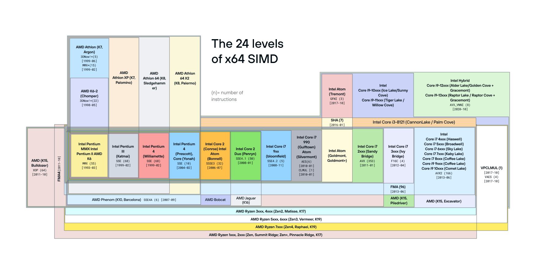
In other words, instead of having a separate implementation for every one of dozens of x86 core designs across Intel, AMD, and Centurion, SimSIMD selects several “capability levels” named after the first server-side CPU line-up that supports a specific family of instructions: Sapphire Rapids for AVX512-FP16, Genoa for AVX-512BF16, Ice Lake for VNNI/VBMI and other AVX-512 integer-processing instructions, Skylake-X for basic AVX-512 support, Haswell for AVX2, F16C, and FMA, etc.

The next step is to map supported CPU features into our “capability levels”:

1
2
3
4
5

   unsigned supports_haswell = supports_avx2 && supports_f16c && supports_fma;
   unsigned supports_skylake = supports_avx512f;
   unsigned supports_ice = supports_avx512vnni && supports_avx512ifma && supports_avx512bitalg && supports_avx512vbmi2 && supports_avx512vpopcntdq;
   unsigned supports_genoa = supports_avx512bf16;
   unsigned supports_sapphire = supports_avx512fp16;

This approach won’t work on Arm. On Arm and Linux, again we can query CPU registers, but on Apple devices we must query the OS. The process is no less convoluted than with x86.

 1
 2
 3
 4
 5
 6
 7
 8
 9
10
11
12
13
14
15
16
17
18
19
20
21
22
23
24
25
26
27

simsimd_capability_t simsimd_capabilities_arm(void) {
#if defined(SIMSIMD_DEFINED_LINUX)
   unsigned long id_aa64isar0_el1 = 0, id_aa64isar1_el1 = 0, id_aa64pfr0_el1 = 0, id_aa64zfr0_el1 = 0;
   __asm__ __volatile__("mrs %0, ID_AA64ISAR0_EL1" : "=r"(id_aa64isar0_el1));
   unsigned supports_integer_dot_products = ((id_aa64isar0_el1 >> 44) & 0xF) >= 1;
   __asm__ __volatile__("mrs %0, ID_AA64ISAR1_EL1" : "=r"(id_aa64isar1_el1));
   unsigned supports_i8mm = ((id_aa64isar1_el1 >> 52) & 0xF) >= 1;
   unsigned supports_bf16 = ((id_aa64isar1_el1 >> 44) & 0xF) >= 1;
   __asm__ __volatile__("mrs %0, ID_AA64PFR0_EL1" : "=r"(id_aa64pfr0_el1));
   unsigned supports_sve = ((id_aa64pfr0_el1 >> 32) & 0xF) >= 1;
   unsigned supports_fp16 = ((id_aa64pfr0_el1 >> 20) & 0xF) == 1;
   if (supports_sve) // Querying SVE2 and SVE2.1 requires SVE to be supported
       __asm__ __volatile__("mrs %0, ID_AA64ZFR0_EL1" : "=r"(id_aa64zfr0_el1));
  
   unsigned supports_sve_i8mm = ((id_aa64zfr0_el1 >> 44) & 0xF) >= 1;
   unsigned supports_sve_bf16 = ((id_aa64zfr0_el1 >> 20) & 0xF) >= 1;
   unsigned supports_sve2 = ((id_aa64zfr0_el1) & 0xF) >= 1;
   unsigned supports_sve2p1 = ((id_aa64zfr0_el1) & 0xF) >= 2;
   unsigned supports_neon = 1; // NEON is always supported on our target platforms


   ....
#elif defined(SIMSIMD_DEFINED_APPLE)
   ...
#else // SIMSIMD_DEFINED_LINUX
   return simsimd_cap_serial_k;
#endif

Feature resolution (like the CPUID above) is great, but it can be slow, sometimes even up to 300 CPU cycles. So you should only do it once, and cache the list of available CPU capabilities.

Conclusion

As you can see, SIMD is full of challenges! And keep in mind, this is just one simple case of us calculating a cosine distance.

But it’s worth it. When one navigates the hurdles and harnesses SIMD correctly, it unlocks incredible performance, often an order of magnitude higher than naive serial code.

I hope you enjoyed this whirlwind tour of SIMD’s complexities! It was quite long, but we didn’t even try analyzing port utilization for different families of instructions on x86. We haven’t looked into SME and streaming SVE modes for recent arm cores. We didn’t study the CPU frequency scaling license, even though many of those aspects are already covered by SimSIMD kernels running under the hood of your favorite data products. So much is still ahead!

In Part 2, we’ll talk about how Mojo helps with a lot of these problems! Ping me (@ashvardanian) or anyone related (@verdagon, @lemire, @clattner_llvm) if you have any questions, and join the Modular Discord server if you have special requests for Part 2!