Scaling-Up Contrastive Learning over NVLink Multicast

It’s 2026, and the world still trains AI models much the way it did when I bought my first Titan V almost a decade ago. Volta had just introduced Tensor Cores, and 16-bit matrix multiplications into 32-bit accumulators were all the rage. PyTorch was only starting to catch up with TensorFlow, and Mellanox was still an independent company selling the InfiniBand cards that joined supercomputers. Since then, Nvidia has bought Mellanox and folded the network into the GPU, but most training code still treats it as an afterthought. What I believe we still don’t do enough is design software around scale-up networks.

There are three ways to scale a GPU workload, and the lines between them are blurry.

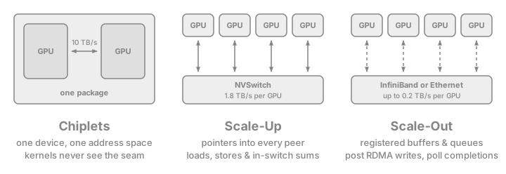
My favorite has always been squeezing more out of every chip, and everyone knows scale-out, adding more servers on a network. But the one in between is the most interesting: a few racks of GPUs talking to each other directly, with remarkable throughput, low latency, and networking primitives built into the hardware. The GPU world calls it scale-up, though I’d call it diagonal, as it adds more chips like scale-out while they still work like one machine. I believe it’s the most important way to scale software these years, and the one least compatible with traditional frameworks like PyTorch or JAX.

That’s the bet behind the upcoming UForm v4 models from Unum: trained around NVL72 pods, where 72 GPUs share one NVLink domain, and built as one model for every modality, rather than separate towers tied together at the top, the way OpenAI’s CLIP and our past UForm models work. So before the release, one simple question:

how much does designing for NVLink actually buy you?

Hardware

I’m pretty much the worst customer a cloud can have: relatively poor, full of hardware demands, and running concurrent RDMA experiments that can stall a machine and every GPU in it. That kind of R&D barely fits on a VM, and even on bare metal it needs machines reconfigured mid-experiment by a patient, hands-on infrastructure team. So for this round, I went to Emma, one of our portfolio companies at AAL VC, and picked two bare-metal boxes of 8× Nvidia B300 SXM6 GPUs:

• Inside each box, the eight GPUs share one NVSwitch with multicast: the scale-up network.
• Between the boxes, each GPU reaches its counterpart through one 100 Gb/s RoCE v2 port: the scale-out network, kept deliberately lean by using one of the four ports each ConnectX-8 card exposes.

Bird’s Eye View & the Results

As usual, let’s start with the dessert!

I wrote a contrastive loss, the kind that trains retrieval and perception embedding models from OpenAI’s CLIP to Google’s SigLIP, as one C++ header and one benchmark binary, where one host thread drives all eight GPUs of a box. Each GPU scores its $R$ rows of 1024-dimensional BFloat16 embeddings against every row on every GPU, at five Matryoshka prefixes.

It competes with the losses people actually train with, all differentiating the same prefixes:

• ScalingContrasts: multimem PTX through the NVSwitch inside a box, RDMA verbs between boxes, and tcgen05 tensor-core tiles for the products.
• open_clip: SigLIP and CLIP losses under PyTorch, with NCCL passing chunks between neighbours, all-gathering them, or all-gathering with gradients for the softmax InfoNCE of CLIP, and cuBLAS for the products.
• big_vision: Google’s SigLIP under jax.jit, where XLA shards it over every GPU and lowers its gathers to NCCL and its products to cuBLAS.

Each cell shows the best loss-step time, then memory per GPU.

On one box, where NVLink joins all eight GPUs:

On two boxes, one process each, joined by the RoCE rails:

ScalingContrasts is the fastest at every size, keeps the same pace per GPU on two boxes as on one at the largest batch, and its memory barely grows as GPUs are added. It’s an apples-to-oranges comparison on purpose: part of that gap comes from engineering, and part from a different loss shape, reflecting how embedding models have moved from two towers toward one since the early 2020s.

One Set or Two

A contrastive loss places matching things close and everything else far, in one embedding space. CLIP turns each row of cosines into a softmax over the batch, while SigLIP scores every cell on its own, with a learned temperature $t$ and bias $b$:

$$\mathcal{L} = -\frac{1}{N} \sum_{i} \sum_{j} \log \sigma\big(z_{ij} \cdot (t \cdot \cos(x_i, y_j) + b)\big)$$

where $z$ is +1 for a positive pair and -1 for every negative. Because every cell stands alone, the grid can be cut into tiles in any order. Matryoshka representations ask the first 64, 128, 256 and 512 dimensions to work as embeddings too, so the cost is five grids, not one.

Every negative a row sees is a row some other GPU computed, and more negatives make better embeddings. So the loss is not a function that happens to be distributed: the loss is the collective, and how much it exchanges depends on its shape:

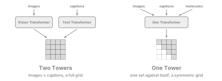
In CLIP and SigLIP’s two-set losses, cells $(i, j)$ and $(j, i)$ pair different images with different captions, and each gradient has two owners, usually on different GPUs. My loss scores one set against itself, with the same labels and weights for mirrored cells, so the owner of row $i$ differentiates both: no embedding gradients cross GPUs. In UForm, an image and its caption are simply two rows of that set marked as a positive pair, which keeps the grid symmetric. The price is scoring every pair twice, once on each owner’s GPU, so at $R = 16384$ on eight GPUs, ScalingContrasts leads big_vision 2.7× in scored cells per second, but 1.36× in distinct pairs.

Part of that lead is plain engineering that any loss could adopt, and the rest is the shape of the loss: embeddings still travel, but their gradients never make the return trip. That’s the point of the whole article: the loss you can afford depends on the network you design for.

I’m not alone in walking that way:

• FuseLIP runs one early-fusion transformer, trained with SigLIP’s sigmoid loss.
• Qwen3-VL-Embedding and GTE add query-query and document-document negatives.
• CLIPPO and OneR use one tower for every modality, with a two-set loss.

On the memory side, DisCo-CLIP and Inf-CL share my instinct to never materialize the whole grid, and SigLIP’s own chunked loss swaps all-gathers for neighbour permutes. ScalingContrasts tiles the same way, but it stages peers over NVLink, and its embedding gradients stay home.

Down the Stack

So what makes such a loss cheap on a scale-up network? The answer follows the diagram from the start, from the inside out: the chip, the box, the switch, and the link between boxes.

On the Chip: Tensor Memory & the Matryoshka Sweep

Blackwell moved the tensor core’s accumulator into a dedicated 256 KB per SM, Tensor Memory, driven by tcgen05 instructions a single thread issues. The forward kernel accumulates every cell’s full 1024-dimensional dot product there, then sweeps back down, subtracting dimensions 512 to 1023, then 256 to 511, 128 to 255 and 64 to 127, so the five prefixes come out widest first. That order lets each band’s gradient build up as a running sum in tensor memory, while the MMA warp sweeps the next segment, so no Float32 cube of products ever reaches HBM. The subtraction comes from the hardware: every tcgen05.mma takes a 32-bit instruction descriptor, and its bit 13 negates the A operand, so the same MMA subtracts instead of adding:

1
2
3
4
5
6

constexpr std::uint32_t forward_negated_instruction_k = forward_instruction_k | (1u << 13); // A negated

// Segment 0 adds every channel, each later segment takes one band back off, widest first.
if (segment == 0) return {0, ladder.ends[widest] / forward_depth_k, forward_instruction_k};
return {ladder.ends[widest - segment] / forward_depth_k, ladder.ends[widest - segment + 1] / forward_depth_k,
        forward_negated_instruction_k};

The surprise was where the time went. The tensor cores finish the products quickly, but every cell of every prefix then needs scalar math on ordinary CUDA cores: normalizing the cosine, the sigmoid, the logarithm and the gradient. That arithmetic, not the MMAs, held the kernel to an eighth of the tensor cores’ peak. Multiplying by stored inverse norms instead of dividing twice per cell, replacing log1pf with a degree-8 polynomial fit, and folding the per-tile partials in parallel made the whole step 1.8× faster.

Across the Box: Pointers, Not Gathers

Inside a box, every GPU maps every other GPU’s memory, and a load from a peer is just a load: NVLink is a memory bus pretending to be a network. So there is no all-gather: each GPU walks its peers one candidate block at a time, staging each over NVLink, as the copy engine feeding the tiles, the Tensor Memory Accelerator (TMA), reads only local memory, and scoring it before touching the next. At fixed $R$, the loss reuses its scratch for every peer, and as each row’s owner differentiates both mirrored cells, its embedding gradient never leaves its GPU.

PyTorch’s DDP and FSDP, Megatron, and most NCCL setups reserve a process or thread per GPU, which in my experience turns synchronization and graph capture into a nightmare once a network pushes sparsity beyond mixture-of-experts. Here one thread enqueues the within-box step for all eight GPUs and never waits on any of them:

1
2
3
4
5
6
7
8

for (gpu_t &gpu : cluster.gpus) {
    gpu.loss.begin(gpu.embeddings.view(), gpu.stream);
    for (gpu_t const &peer : cluster.gpus) // a peer's embeddings are just a pointer
        gpu.loss.score(gpu.embeddings.span(), peer.embeddings.view(), gpu.local() * rows,
                       peer.local() * rows, beta, bias, live, gpu.stream);
    gpu.loss.finish(gpu.embeddings.view(), gpu.gradient.span(), domain.payload(gpu.local()), gpu.stream);
    domain.all_reduce(gpu.local(), summand_scalars_k, gpu.stream);
}

Yes, this is what modern C++ looks like if you use NumKong tensors 😉 If you want, you can even wrap the multicast memory from the next section into a custom allocator that hands every GPU the same offset in its own copy, so a buffer mirrored across GPUs becomes just another nk::tensor<f32_t, multimem_allocator<f32_t>, 1>, where nk::tensor is a memory-owning analog of std::mdspan.

Ordering inside the box comes only from device barriers, so the host never waits for GPU completion. It’s not free, though: the thread enqueues about 55 calls per GPU, and the last GPU starts so late that the final all-reduce spends almost 40% of a mid-sized step waiting. CUDA Graphs should remove the skew, but the cross-box path still blocks the thread on RDMA completions, and the learned temperature and bias still arrive as host floats.

Spinning has a nastier trap. With lazy loading, the first launch of a kernel can block the host thread on device synchronization. A device spinning in a barrier, for a peer the thread hasn’t reached yet, never goes idle, so nothing crashes and the step never ends. Loading every kernel on every GPU before the first barrier fixes it.

In the Switch: Barriers & Reductions

Since Hopper, the NVSwitch can add numbers in flight, NVLink SHARP in Nvidia’s words, exposed in PTX as multimem instructions on one address mapped to every GPU. Our loss sums only three scalars this way, but a real training step sums every weight gradient, with the same all-reduce:

1
2
3
4
5

f32_t x, y, z, w; // one switch-reduced load sums 4 scalars across all 8 GPUs
asm volatile("multimem.ld_reduce.relaxed.sys.global.add.v4.f32 {%0, %1, %2, %3}, [%4];"
             : "=f"(x), "=f"(y), "=f"(z), "=f"(w) : "l"(&multicast[scalar]) : "memory");
asm volatile("multimem.st.relaxed.sys.global.v4.f32 [%0], {%1, %2, %3, %4};"
             :: "l"(&multicast[scalar]), "f"(x), "f"(y), "f"(z), "f"(w) : "memory");

It moves 1.3× the best bus bandwidth I measured with NCCL, repeats bit for bit, and keeps its rounds on the device, so a replay needs no host writes.

But the switch ends at the edge of the box.

Between Boxes: One Write per Embedding

Past it, each GPU writes its embeddings straight into its counterpart’s memory through its own RoCE port, once per step, while both boxes score their own blocks. Every byte that leaves a GPU has to earn its trip, and each trip is one work request:

1
2
3
4
5
6
7
8

ibv_sge piece {source, std::uint32_t(bytes), source_key};
ibv_send_wr request {}, *refused = nullptr;
request.sg_list = &piece, request.num_sge = 1;
request.opcode = IBV_WR_RDMA_WRITE_WITH_IMM; // lands in the peer's GPU memory, then wakes its queue
request.send_flags = IBV_SEND_SIGNALED;
request.imm_data = htonl(std::uint32_t(bytes));
request.wr.rdma.remote_addr = target, request.wr.rdma.rkey = target_key;
require(ibv_post_send(queue_pair, &request, &refused), "write posting");

Without the nvidia_peermem module, GPU memory registers with the NIC as a dma-buf, and the scatter entry must name the device pointer, not the address the registration returns, or the first write dies with “local protection error”.

Footprint

Going this deep has a side benefit: the binaries get much smaller, so a training pipeline doesn’t have to start with an hour-long Docker pull:

• cuBLAS with cuBLASLt: 603 MB, 45× larger, just for the matrix products.
• NCCL: 242 MB, 18× larger, just for the collectives.
• NVSHMEM: 78 MB, 6× larger, just for the symmetric memory.
• ScalingContrasts: 13.4 MB for the tiles, the peer staging, the switch collectives and the rails, plus the CUDA driver, a 0.8 MB libcudart and libibverbs.

The catch is that those 13.4 MB target exactly one GPU model, and the machines coming next may each need a binary of their own.

The Future of Scale-Up

The scale-up domain is growing beyond an eight-GPU box, and Nvidia isn’t the only vendor building it. Across vendors and generations, the whole machine changes shape:

So, how much does designing for NVLink buy you? On two B300 boxes, a one-set loss built around the switch runs 2.9× faster than big_vision’s two-tower SigLIP, holds 35× less memory per GPU, and keeps its per-GPU pace from one box to two. And if you’re buying Rubin, it’s a different platform and a different binary, but this may be the first generation in years where the source can stay the same: Hopper’s wgmma gave way to Blackwell’s tcgen05 and tensor memory, while Rubin seemingly keeps both, along with the multimem reductions in its NVLink 6 switches. The CUDA implementation and the PyTorch & JAX baselines are on GitHub, if you want to try it.