In this fourth article of the “Less Slow” series, I’m accelerating Unum’s open-source Vector Search primitives used by some great database and cloud providers to replace Meta’s FAISS and scale-up search in their products. This time, our focus is on the most frequent operation for these tasks - computing the the Cosine Similarity/Distance between two vectors. It’s so common, even doubling it’s performance can have a noticeable impact on applications economics. But compared to a pure Python baseline our single-threaded performance grew by a factor of 2'500x. Let’s go through optimizations one by one:
- Kicking off with basic Python.
- Noticed a 35x slowdown when not using NumPy right.
- Managed a 2-5x speed boost with SciPy.
- Jumped to a 200x speedup using C.
- A big leap to 400x faster with SIMD intrinsics.
- Touched 747x combining AVX-512 and BMI2.
- Climbed to 1,260x adding AVX-512FP16.
- The final high: 2,521x faster with AVX-512VNNI.
Some highlights:
- Again,
gotodoesn’t get the love it deserves in C. - BMI2 instructions on x86 are consistently overlooked… thanks to AMD Zen2, I guess.
- AVX-512FP16 is probably the most important extension in the current AI race.
I’m still scratching my head on the 4VNNI extensions of AVX-512, and couldn’t find a good way to benefit from them here or even in the polynomial approximations of the Jensen Shannon divergence computations in the last post, so please let me know where I should try them 🤗
Cosine Similarity
Cosine Similarity is a way to check if two “vectors” are looking in the same direction, regardless of their magnitude. It is a widespread metric used in Machine Learning and Information Retrieval, and it is defined as:
$$ \cos(\theta) = \frac{A \cdot B}{|A| |B|} = \frac{\sum_{i=1}^{n} A_i B_i}{\sqrt{\sum_{i=1}^{n} A_i^2} \sqrt{\sum_{i=1}^{n} B_i^2}} $$
Where $A$ and $B$ are two vectors with $n$ dimensions. The cosine similarity is a value between $-1$ and $1$, where $1$ means that the two vectors are pointing in the same direction, $-1$ implies that they are pointing in opposite directions and $0$ means that they are orthogonal. Cosine Distance, in turn, is a distance function, which is defined as $1 - \cos(\theta)$. It is a value between $0$ and $2$, where $0$ means that the two vectors are identical, and $2$ means that they are pointing in opposite directions. I may use the terms interchangeably, but they are not exactly the same.
Python
The first implementation is the most naive one, written in pure Python… by ChatGPT. It is a direct translation of the mathematical formula and is very easy to read and understand.
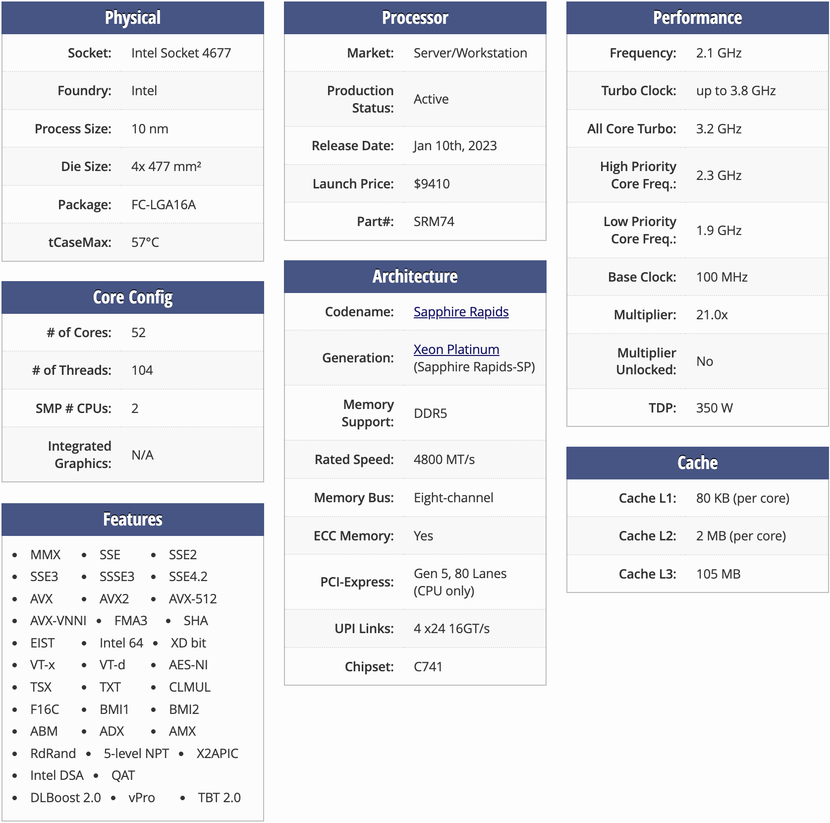
I’ll run on 4th Gen Intel Xeon CPUs, codenamed Sapphire Rapids, and available on AWS as the r7iz instances. Before running a benchmark, let’s generate random numbers and put them into a list, simulating the 1536-dimensional “embeddings” from the OpenAI Ada service.
Running the benchmark with the %timeit utility, we get 93.2 µs ± 1.75 µs per loop.. Or roughly 100 microseconds per call. Is that good or bad?
Our solution is Pythonic but inefficient, as it traverses each list twice. So let’s use the common Pythonic zip idiom:
Running the benchmark, we get 65.3 µs ± 716 ns per loop., resulting 30% savings! I believe it’s a fair baseline.
As pointed on HackerNews, I forgot to apply the square root for
magnitude_aandmagnitude_b.
NumPy: Between Python and C
NumPy is a powerful tool in Python’s toolbox, helping folks work fast with arrays. Many people see it as the go-to for doing science stuff in Python. A lot of machine learning tools lean on it. Since it’s built with C, you’d think it’d be speedy. Let’s take our basic Python lists and make them sharper with NumPy. We’re looking at single-precision, half-precision numbers, and 8-bit integers.
These are popular choices for quantization (making data smaller) in tools like Meta’s FAISS and Unum’s USearch. Half-precision is pretty handy, working well most of the time. But using integers? That depends on the AI model you’re using. Thanks to Quantization Aware Training, two of my faves — Microsoft’s E5 for just text and Unum’s UForm for multi-modal data — work well even compressed to 8-bit numbers.
After getting our vectors set up, I used our cosine_distance function to see how similar the three arrays are:
floats: 349 µs ± 5.71 µs per loop.halfs: 525 µs ± 9.69 µs per loop.ints: 2.31 ms ± 26 µs per loop.
But here’s the problem. Instead of getting faster, things went 35x slower than our 65.3 µs starting point. Why?
Memory Management: Sure, NumPy uses C arrays, which are cool. But every time we loop through them, we turn small byte stuff into bigger Python stuff. And with memory being unpredictable, it’s surprising things didn’t go even slower.
Half-Precision Support: Most new devices support half-precision. But the software side? Not so much. Only a few AI tools use it, and they often focus on GPU stuff, leaving out the CPU. So, converting half-precision things on the go can be slow.
Integer Overflows: Doing math with our tiny integers isn’t smooth. We keep getting these annoying overflow warnings. The CPU spends more time checking things than actually doing the math. We often see things like: “RuntimeWarning: overflow encountered in scalar multiply”.
Here’s a tip: If you’re using NumPy, go all in. Mixing it with regular Python can really slow you down!
SciPy
NumPy is also the foundation of the SciPy library, which provides many valuable functions for scientific computing, including the scipy.distance.spatial.cosine. It will use the native NumPy operations for as much as possible.
floats: 15.8 µs ± 416 ns per loop.halfs: 46.6 µs ± 291 ns per loop.ints: 12.2 µs ± 37.5 ns per loop.
Now, we see the true potential of NumPy, and the underlying Basic Linear Algebra Subroutines (BLAS) libraries implemented in C, Fortran, and Assembly. Our pure Python baseline was 65.3 µs, and we now got 2-5 times faster, depending on the data type. Notably, halfs are still slow. Checking the specs of a similar CPU, we can clearly see support for f16c instructions, which means that the CPU can at least decode half-precision values without software emulation, and we shouldn’t be experiencing this much throttling.
C
C is the lowest-level hardware-agnostic programming language - hence the best way to optimize small numerical functions, like the Cosine Similarity and Distance.
It is also trivial to wrap C functions into pure CPython bindings for the default Python runtime, and if you use the FastCall convention, like we do, you can make your custom code as fast as the built-in Python functions, like what I’ve described recently with StringZilla, replacing Python’s default str string class with a faster alternative.
Unlike C++, however, C doesn’t support “generics” or “template functions”.
So we have to separately implement the cosine_distance function for each data type we want to support, or use the ugly “macros”:
| |
This is a real snippet from the library and depends on yet another macro - SIMSIMD_RSQRT(x), defined as the 1 / sqrtf(x) by default.
We later instantiate it for all the data types we need:
Those macros will generate the following functions:
simsimd_serial_f32_cos: for 32-bitfloats.simsimd_serial_f16_cos: for 16-bithalfs, accumulating 32-bit values.simsimd_serial_i8_cos: for 8-bitints, accumulating 32-bit values.
We benchmark those using the Google Benchmark library:
floats: 1956 ns ~ 33x faster than Python.halfs: 1118 ns ~ 58x faster than Python.ints: 299 ns ~ 218x faster than Python.
That’s a great result, but this code relies on the compiler to perform heavy lifting and produce efficient Assembly. As we know, sometimes even the most recent compilers, like GCC 12, can be 119x slower than hand-written Assembly. Even on the simplest data-parallel tasks, like computing the Jensen Shannon divergence of two discrete probability distributions.
I’ve found a fairly simple data-parallel workload, where AVX-512FP16 #SIMD code beats O3/fast-math assembly produced by GCC 12 by a factor of 118x 🤯🤯🤯https://t.co/cFftGbMBQe
— Ash Vardanian (@ashvardanian) October 23, 2023
Assembly
Assembly is the lowest-level programming language, and it is the closest to the hardware. It is also the most difficult to write and maintain, as it is not portable, and it is very easy to make mistakes. But it is also the most rewarding, as it allows us to write the most efficient code and to use the most advanced hardware features, like AVX-512. AVX-512, in turn, is not a monolith. It’s a very complex instruction set with the following subsets:
- AVX-512F: 512-bit SIMD instructions.
- AVX-512DQ: double-precision floating-point instructions.
- AVX-512BW: byte and word instructions.
- AVX-512VL: vector length extensions.
- AVX-512CD: conflict detection instructions.
- AVX-512ER: exponential and reciprocal instructions.
- AVX-512PF: prefetch instructions.
- AVX-512VBMI: vector byte manipulation instructions.
- AVX-512IFMA: integer fused multiply-add instructions.
- AVX-512VBMI2: vector byte manipulation instructions 2.
- AVX-512VNNI: vector neural network instructions.
- AVX-512BITALG: bit algorithms instructions.
- AVX-512VPOPCNTDQ: vector population count instructions.
- AVX-5124VNNIW: vector neural network instructions word variable precision.
- AVX-5124FMAPS: fused multiply-add instructions single precision.
- AVX-512VP2INTERSECT: vector pairwise intersect instructions.
- AVX-512BF16:
bfloat16instructions. - AVX-512FP16: half-precision floating-point instructions.
Luckily, we won’t need all of them today. If you are curious, you can read more about them in the Intel 64 and IA-32 Architectures Software Developer’s Manual… but be ready, it’s a very long read.
Moreover, we don’t have to write the Assembly per se, as we can use the SIMD Intrinsics to essentially write the Assembly instructions without leaving C.
| |
Let’s start with a relatively simple implementation:
- A single
for-loop iterates through 2 vectors, scanning up to 16 entries simultaneously. - When it reaches the end of the vectors, it uses a mask to load the remaining entries with the
((1u << (n - i)) - 1u)mask. - It doesn’t expect the vectors to be aligned, so it uses the
loaduinstructions. - It avoids separate additions using the
fmaddinstruction, which computesa * b + c. - It uses the
reduce_addintrinsic to sum all the elements in the vector, which is not a SIMD code, but the compiler can optimize that part for us. - It uses the
rsqrt14instruction to compute the reciprocal square root of the sum ofa2andb2, very accurately approximating1/sqrt(a2)and1/sqrt(b2), and avoiding LibC calls.
Benchmarking this code and its symmetric counterparts for other data types, we get the following:
floats: 118 ns ~ 553x faster than Python.halfs: 79 ns ~ 827x faster than Python.ints: 158 ns ~ 413x faster than Python.
We are now in the higher three digits.
BMI2 and goto
The world is full of prejudice and unfairness, and some of the biggest ones in programming are:
- considering a
gototo be an anti-pattern. - not using the BMI2 family of assembly instructions.
The first one is handy when optimizing low-level code and avoiding unnecessary branching. The second is a tiny set of bzhi, pdep, pext, and a few other, convenient for bit manipulation! We will restore fairness and introduce them to our code, replacing double-precision computations with single-precision.
| |
Result for floats: 87.4 ns ~ 747x faster than Python.
One of the reasons the BMI2 extensions didn’t take off originally is that, AMD processors before Zen 3 implemented
pdepandpextwith a latency of 18 cycles. Newer CPUs do it with the latency of 3 cycles.
FP16
Ice Lake CPUs supported all the instructions we’ve used so far. In contrast, the newer Sapphire Rapids instructions add native support for half-precision math.
| |
The body of our function has changed:
- we are now scanning 32 entries per cycle, as the scalars are 2x smaller.
- we are using the
_phintrinsics, the half-precision counterparts of the_psintrinsics.
Result for halfs: 51.8 ns ~ 1'260x faster than Python.
VNNI
Today’s final instruction we’ll explore is the vpdpbusd from the AVX-512VNNI subset. It multiplies 8-bit integers, generating 16-bit intermediate results, which are then added to a 32-bit accumulator. With smaller scalars, we can house 64 of them in a single ZMM register.
| |
After compiling, you might expect to see three vpdpbusd invocations. However, the compiler had other ideas. Instead of sticking to our expected flow, it duplicated vpdpbusd calls in both branches of the if condition to minimize code sections and jumps. Here’s a glimpse of our main operational section:
.L2:
        ; Check `if (n < 64)` and jump to the L7 if it's true.
        cmp     rax, rdx
        je      .L7
        ; Load 64 bytes from `a` and `b` into `zmm1` and `zmm0`.
        vmovdqu8        zmm1, ZMMWORD PTR [rdi]
        vmovdqu8        zmm0, ZMMWORD PTR [rsi]
        ; Increment `a` and `b` pointers by 64.
        add     rdi, 64
        add     rsi, 64
        ; Perform mixed-precision dot-products.
        vpdpbusd        zmm4, zmm1, zmm0 ; ab = b * a
        vpdpbusd        zmm3, zmm1, zmm1 ; b2 = b * b
        vpdpbusd        zmm2, zmm0, zmm0 ; a2 = a * a
        ; Subtract the number of remaining entries and jump back.
        sub     rdx, 64
        jne     .L2
.L7:
        ; Process the tail, by building the `k1` mask first.
        ; We avoid `k0`, which is a hardcoded constant used to indicate unmasked operations.
        mov     rdx, -1
        bzhi    rax, rdx, rax
        kmovq   k1, rax
        ; Load under 64 bytes from `a` and `b` into `zmm1` and `zmm0`,
        ; using the mask from the `k1`, which can be applied to any AVX-512 argument.
        vmovdqu8        zmm1{k1}{z}, ZMMWORD PTR [rdi]
        vmovdqu8        zmm0{k1}{z}, ZMMWORD PTR [rsi]
        ; Perform mixed-precision dot-products.
        vpdpbusd        zmm3, zmm1, zmm1 ; b2 = b * b
        vpdpbusd        zmm4, zmm1, zmm0 ; ab = b * a
        vpdpbusd        zmm2, zmm0, zmm0 ; a2 = a * a
        ; Exit the loop.
        jmp     .L4
It’s often intriguing to see how compilers shuffle around my instructions, especially when it seems somewhat arbitrary in brief code segments. Our heavy SIMD will anyways be decoded into micro-ops, and then the CPU rearranges them all over again, disregarding compiler’s sequence. Still, upon testing this with the Google Benchmark library, we observed the following for ints: 25.9 ns, which is roughly 2'521 times faster than our original Python baseline. Delivered as promised 🤗
Conclusion
There’s a common belief that you need a massive infrastructure, akin to what giants like OpenAI or Google possess, to create impactful technology. However, I’m a proponent of the idea that many amazing innovations can spring from humble beginnings – even on a shoestring budget. If you share this sentiment and are keen on optimizing and innovating, you might be interested in some other libraries I’ve had a hand in. 😉
 |  |  |  |  |
Appendix: Comparing Compilers
For those eager to delve deeper, examining the Assembly generated by different compilers can be insightful. A popular comparison is between GCC and Intel’s new ICX compiler, with the latter now being based on LLVM. Before diving into the Assembly details, let’s first benchmark their performance.
| |
The above script compiles the code using both compilers and then runs each binary, exporting the results into distinct JSON files. Afterwards, you can use Google Benchmark’s lesser-known tool, compare.py, to determine if there are significant performance differences and whether a deeper dive into the Assembly is warranted:
| |
From the results, we observe minimal runtime differences between the two compilers. The generated Assembly is remarkably similar, particularly in the critical sections. Intel’s output is often 10% shorter which is typically advantageous. The most pronounced differences emerge outside of the for loop. Notably, the _mm512_reduce_add_epi32 intrinsic doesn’t correspond directly to a specific SIMD instruction, granting the compilers a bit more leeway:
- GCC opts for a lengthier reduction using
vextracti64x4andvextracti64x2. - Intel prefers the succinct
vextracti128.
Both compilers employ the vpshufd for shuffling but use varied masks. For a detailed exploration, visit the Compiler Explorer.