This will be a story about many things: about computers, about their (memory) speed limits, about very specific workloads that can push computers to those limits and the subtle differences in Hash-Tables (HT) designs. But before we get in, here is a glimpse of what we are about to see.

A friendly warning, the following article contains many technical terms and is intended for somewhat technical and hopefully curious readers.
All the benchmarks can be analyzed in detail and reproduced with the code available on our GitHub page. Everyone is welcome to contribute! And NO, it’s not a single-threaded benchmark. And NO, we aren’t suggesting to replace servers with MacBooks. These and luckily deeper questions were discussed in full here: #4 Ranking HackerNews post, original HackerNews post, r/cpp Reddit community.
A couple of months ago, I followed one of my oldest traditions, watching Apple present their new products at one of its regular conferences.
I have done it since the iPhone 4 days and haven’t missed a single one.
Needless to say, the last ten years were a rodeo.
With hours spent watching new animated poop emojis on iOS presentations, I would sometimes lose hope in that 💲3T company.
After the 2012 MacBook Pro, every following Mac I bought was a downgrade.
The 2015 model, the 2017 and even the Intel Core i9 16" 2019 version, if we consider performance per buck.
Until now.
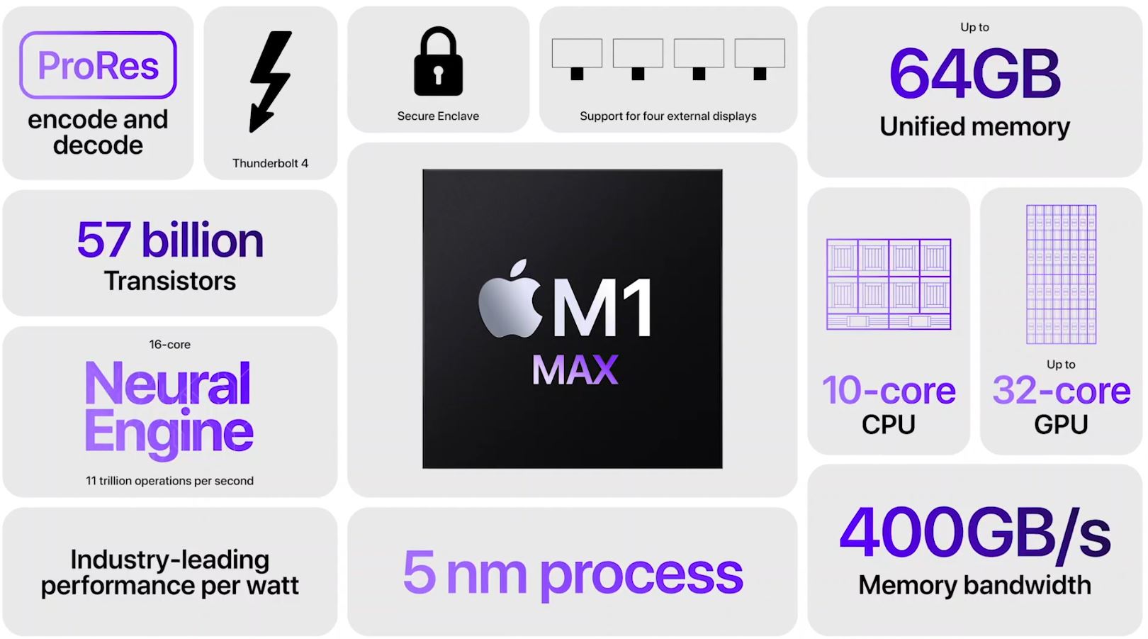
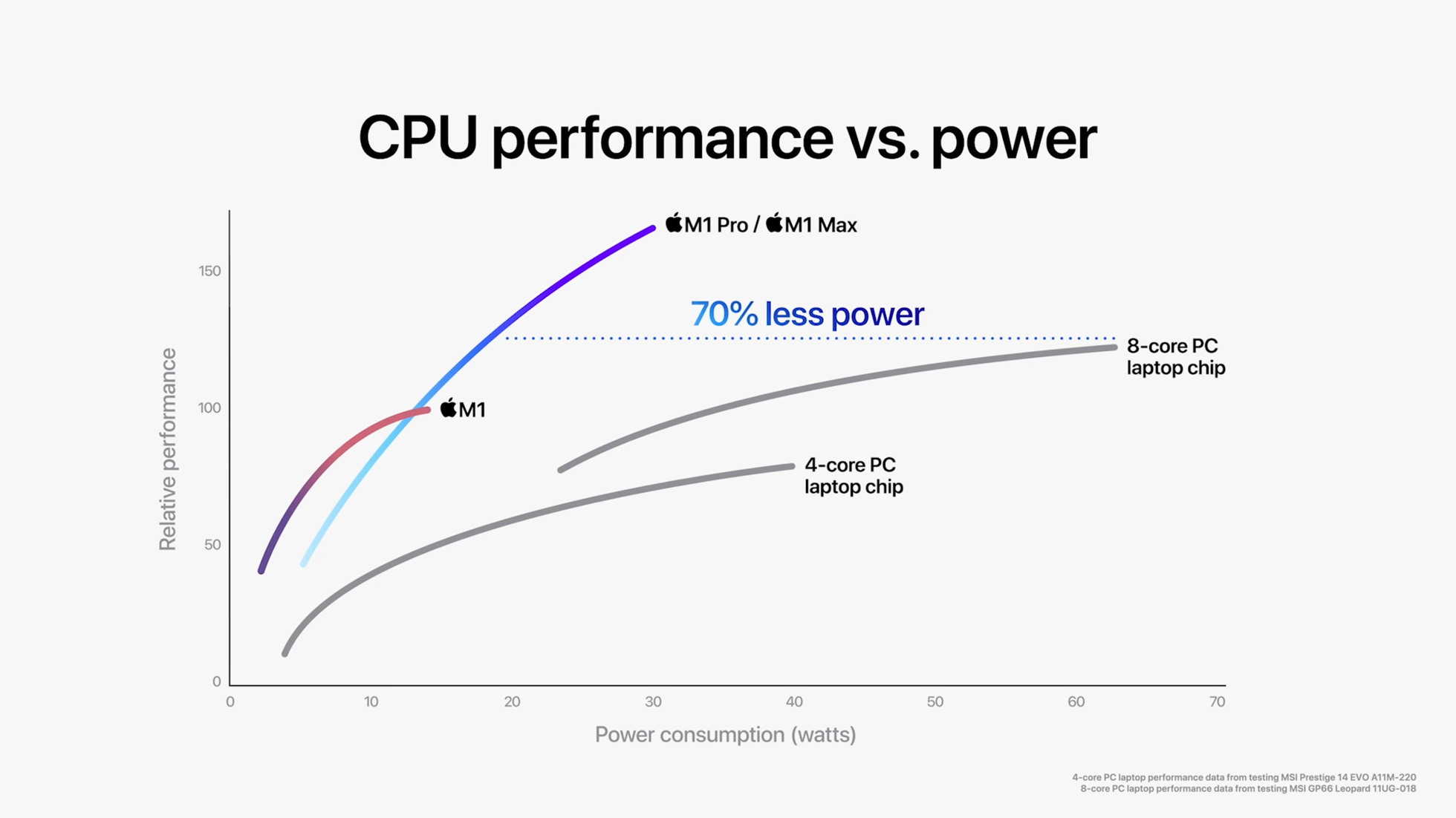
The M1 Pro/Max seem vastly different from the M1 in last year’s MacBook Airs. Apple hates sharing technical details, but here are some of the core aspects we know:
- CPU has 8x power cores and 2x efficiency cores.
- Cores have massive L2 blocks for a total of 28 MB of L2.
- Fabrication was done on TSMC’s N5 process.
- Memory bus was upgraded to LPDDR5 and claims up to 400 GB/s of bandwidth.
We have recently published a 2736-word overview of upcoming memory-bus innovations, so the last one looks exceptionally interesting. In the “von Neumann computer architecture” today, the biggest bottleneck is between memory and compute. It’s especially evident in big-data processing and neuromorphic workloads. Both are essential to us, so we invested some time and benchmarked memory-intensive applications on three machines:
- 16" Apple MacBook Pro with an 8-core Intel Core i9-9980HK and 16 GB of DDR4 memory, purchased for around 💲3'000 in 2019.
- 16" Apple MacBook Pro with a 10-core ARM-based M1 Max CPU with 64 GB of LPDDR5 memory, purchased for around 💲3'000 in 2021.
- A custom-built liquid-cooled server with an AMD Threadripper Pro 3995WX with 1 TB of eight-channel DDR4 memory, purchased for over 💲50'000 in 2021. Its full description can be found in our previous article on the Yahoo Cloud Serving Benchmark. Spoiler, it’s 🌰🌰🌰.
Sounds intriguing? Let’s jump in!
Copying Memory
Generally, when companies claim a number like 100 GB/s, they mean the combined theoretical throughput of all the RAM channels in the most basic possible workload - sequentially streaming a lot of data.
Probably the only such use case on a desktop is watching multiple 4K movies at once.
Your multimedia player will fetch a ton of frames from memory and put them into the current frame buffer, overwriting the previous content.
In the x86 world, you would achieve something like that by combining _mm256_stream_load_si256 and _mm256_stream_si256 intrinsics.
Or if you prefer something higher-level, there is a memcpy in every libc distribution.

In this benchmark, we generated a big buffer with lots of synthetic random data in it, and then every core would fetch chunks of it in random order. As we see, there is much non-uniformity in the results. The evaluation speed may differ significantly depending on the copied chunk size (1 KB, 4 KB, 1 MB or 4 MB). The expectation is that copies below 4 KB standard page size won’t be efficient. As you make chunks bigger, the numbers would generally increase until reaching about 200 GB/s in copied data on the newest hardware. All of that bandwidth, of course, rarely affects real life.
- If you are watching videos - you are likely decoding → bottlenecking on CPUs ALUs.
- If you handle less than 20 MB at a time → you may never be leaving CPUs L1/L2 caches.
Is there a memory-intensive benchmark that can translate into real-world performance?
Hash-Tables
Meet Hash-Tables (HT) - probably the most straightforward yet most relevant data structure in all computing. Every CS freshman can implement it, but even the biggest software companies in the world spend years optimizing and polishing them. Hell, you can build a 💲2B software startup like Redis on a good hash-table implementation. That’s how essential HTs are! In reality, HT is just key-value store implemented as a bunch of memory pockets and an arbitrary mathematical function that routes every key to a bucket in which that data belongs. The problem here, is that generally a tiny change in input data results in a jump to a different memory region. Once it happens, you can’t fetch the data from the CPU caches and have to go all the way to RAM! So our logic is the following:
- Fast memory → Fast Hash-Tables.
- Fast Hash-Tables → Faster Applications.
- Faster Applications → 🌈 Rainbows, 🦄 Unicorns and 🤑 Profit!
With this unquestionable reasoning in mind, let’s compare some hash-tables on Apple’s silicon!
C++ Standard Templates
The most popular high-performance computing language is C++, and it comes with a standard library. A standard library with many zero-cost abstractions, including some of the fastest general-purpose data structures shipped in any programming ecosystem. It’s the most common HT, the people will be using, but not the fastest.
We have configured it in all power-of-two sizes between 16 MB and 256 MB of content. Such a broad range is selected to showcase speeds both within and outside of CPU caches of chosen machines.

Wow! What we see here, is that ARM-powered MacBooks end-up fetching about 6 GB/s worth of data. That of course, is nowhere close to the 100 GB/s in bulk-copy-workloads or 400 GB/s on the slide, but remarkably close to a huge server and way ahead of the last gen Intel chip!
Implementation-wise, STL std::unordered_map is an array of buckets, where every bucket is a linked list.
Every node of those linked lists is allocated in a new place on the heap in the default configuration.
Once we get a query, we hash the key, determine the bucket, pick the head of the list and compare our query to every object in the list.
This already must sound wasteful in the number of entries we will traverse.
Then, a linked list in each bucket would require storing at least one extra eight-byte pointer per added entry. If you are mapping integers to integers, you will be wasting at least half of the space in the ideal case. Continuing the topic of memory efficiency, allocating nodes on-heap means having even more metadata about your HT stored in another tree data structure. Let’s take the second most popular solution.
Google Hash Maps
Googles SparseHash library as over ⭐ 1K on GitHub!
They have a sparse and a dense google::dense_hash_map HT, the latter one being generally better across the board.
Googles design is based on the idea of open-addressing.
Instead of nesting linked-lists in every bucket, they keep only one plain memory buffer.
If a slot is busy, a linear probing procedure is called to find an alternative.
This methodology has a noticeable disadvantage.
Previously, with std::unordered_map we could allocate one entry at a time, making memory consumption higher but more predictable.
Here, we have a single big arena, and when it’s 70% populated, we generally create another one, double the size, and migrate the data in bulk.
Sometimes, for 7x entries, we will use 30x worth of memory over four times what we expected.
Furthermore, those bulk migrations don’t happen momentarily and will drastically increase the latency on each growth. This HT performs better on average but lowers predictability and causes latency spikes.
Another disadvantage with this library is defining an “empty key”. If your integer keys are only 4 bytes in size, this means reserving and avoiding 1 in 4'000'000'000 potential values. A small functional sacrifice in most cases, but not always.
TSL Library
If you feel a little less mainstream and curious to try other things, tsl:: is another interesting namespace to explore.
Its best solution also relies on open addressing but with a different mechanism of probing and deletion.

Best of all, the author provides numerous benchmarks, comparing his tsl::robin_map to some of the other established names.
At Unum, however, we don’t use any third-party HT variants. In this article, we only benchmarked a single operation - a lookup. A broader report would include: insertions, deletions and range-constructions, to name a few and would highlight broader tradeoffs between different pre-existing solutions.

When those benchmarks are running, we disable multithreading, pin cores to the process, start a separate sub-process that queries the system on both software and hardware events, like total reserved memory volume and the number of cache misses. Those benchmarks run on Intel, AMD and ARM CPU design, on machines ranging from 3 W to 3 kW power-consumption, running Linux and sometimes even macOS, as we saw today.
In years of High-Performance Computing Research, you learn one thing - there are no absolute benchmarks. Noise and fluctuations are always present in the results. Still, with gaps this obvious, we are genuinely excited about Apple’s new laptops and can’t wait for the next generation of servers to adopt DDR5 technology!
Continue reading on this topic:
Or check out my GitHub for more interesting projects.